William Rainey Harper College
ECO 211
Microeconomics: An Introduction to Economic Efficiency

ASSIGNMENTS

LESSONS

~/~ Practice Exercises ~/~ Video Lecture Notes ~/~ Textbook Website ~/~ Blackboard ~/~ Old Lecture Outlines

For due dates see the SCHEDULE link on Blackboard


UNIT 1: Introduction to Microeconomics
1a - 1b - 1c - 1d - 2a - 3a - 3b - 3c - 5a - 5b

UNIT 2: Elasticity, Consumer Choice, and Costs
4a - 4b - 6a - 7a - 7b - 7c

UNIT 3: Product Markets and Efficiency
8/9a - 8/9b - 10a - 10b - 11a - 11b

UNIT 4: Resource Markets, Inequality, and Immigration
12a - 13a - 20a - 22a

Unit 1: INTRODUCTION TO MICROECONOMICS

1a  Day One

Welcome to ECO 211! My name is Mark Healy. I will be your economics instructor for the semester. Please call me "Mark".
Many students end up dropping or failing this course due to the lack of basic math skills. If your math skills are weak you should consider building them before taking this course. If you are required to take MTH 055 and have not yet done so, do not take this economics course until you have successfully completed it. The face-to-face sections will take a practice math quiz on the first day of class. For the online section I have posted the math quiz on our Blackboard site. Take the math quiz on Blackboard or in class. If you score less then 14 or 15, consider dropping ECO 211 and taking a math class first.

Topics:

  • math quiz
  • syllabus/orientation

Readings:

Video Lectures: [Cengage login] [TW login] [notes]

Discussion Questions:

  • na

Must Know / Outcomes:

  • basic math skills
  • how to find class information

1b   The 5Es of Economics

The "5Es of Economics" are not from the textbook. I borrowed the concept (with many modifications) from another textbook many years ago. I believe it concisely explains the purpose of economics. Also, it begins to introduce students to the economic way of thinking. The economic problem that we all face, that all countries face, that the world faces, is SCARCITY. Economics is the study of how we can reduce scarcity. What I like about the 5Es model is that it shows us that there are only five ways to reduce scarcity. Only five. Simple.

For each of the 5Es (1) learn the defininition, (2) understand examples, and most importantly, (3) know how they reduce scarcity and help to maximize society's satisfaction.

This is where you learn that it may be good when the price of plywood increases greatly during a hurricane. And it might be good when Coca-Cola lays of one fifth of its workforce. Or, that the price of gasoline may be too low. Really.

Topics:

  • 5Es of Economics
  • algebra and graphs

Readings:

  • Syllabus
  • 5Es online reading (VERY IMPORTANT!)
  • Ch. 3: "Efficient Allocation" pp. 58-59
  • Ch. 3 and 6: "Diminishing Marginal Utility" pp. 49 and 117
  • Ch.1, Appendix on Graphing

Video Lectures: [Cengage login] [TW login] [notes]

Discussion Questions:

  • Why it is GOOD for the people of Florida if, after a hurricane strikes, the price of plywood (or other products) increases from $10 a sheet to $30 a sheet?
  • Why it was GOOD when the Coca-Cola company (or other companies) lays off 6000 workers as they did in the year 2000?
  • Why the price of gasoline in the United States is TOO LOW? (We may have to wait until after we finish chapter 5 to truly understand this.)
  • Explain the "President Obama Example" of how equity increases society's satisfaction.

Must Know / Outcomes:

  • What is "SCARCITY" as it is defined in economics?
    (What two things cause the scarcity of goods and services?
  • What is "erskinite"? Is erskinite scarce?
  • What is the goal of economics? 
  • What are society's three options for dealing with scarcity?
  • What do the 5Es do?
  • For each of the 5Es:
    • Define
    • Explain how it affects society's satisfaction
    • Give an example

    • ECONOMIC GROWTH
    • ALLOCATIVE EFFICIENCY
    • PRODUCTIVE EFFICIENCY
    • EQUITY
    • FULL EMPLOYMENT

  • How does economic growth differ from the other Es? 
  • What are the three ways to achieve economic growth?
  • What are the three ways to achieve productive efficiency?
  • What is the President Obama example? Explain how it can be used to show that equity can increase society's satisfaction. Why did we use such a strange example?
  • What is the law of diminishing marginal utility? What does "marginal" mean?

1c  Scarcity and Budget Lines

So, do you agree that it is GOOD for the people of Florida if, after a hurricane strikes, the price of plywood (or other products) increases from $10 a sheet to $30 a sheet? Or, that it was GOOD when the Coca-Cola company (or other companies) layed off 6000 workers as they did in the year 2000 assuming that they could still produce the same quantity, but with fewer workers? Even if you do not agree, do you understand that these things will reduce scarcity and increase society's satisfaction? In chapter five we will learn why the price of gasoline, soda pop, and junk food, may be TOO LOW. (Isn't this fun?)

Lesson 1c introduces our first graphic MODEL: the budget line. For many students microeconomics is a difficult course. I think there are two reasons for this. First, we will learn therories or models, rather than facts. Facts are easy to memorize. Theories or models have to be learned and practiced. And second, we will express our theories or models on graphs, and many studetns do not like graphs. If you want to be successful you must learn to use our graphical models. You must be able to draw the graphs correctly from memory, you must understand what each line on the graph represents, and you must know why each line has the shape that it does: DEFINE, DRAW, DESCRIBE SHAPE. Study the graphs in the textbook carefully and plot all the graphs in the yellow pages. Finally, remember this: each point on a graph represents two numbers. It is that easy. Find a point on a graph, then find the two number from the graph's axes.

Topics:

  • Definition of econonomics
  • Economic models
  • Budget lines
  • Resources

Readings:

  • Ch 1, pp.1-11

Video Lectures: [Cengage login] [TW login] [notes]

  • WHAT IS ECONOMICS: SCARCITY, THE 5Es, AND MAKING CHOICES
  • BUDGET LINES
    • 6A-1 Constructing a Consumer's Budget Constraint [TW 3.2.1 (9:36)]
    • 6A-2 Understanding a Change in the Budget Constraint [TW 3.2.2 (5:02)]

Discussion Questions:

  • Why do economists use all those graphs (models)?

Must Know / Outcomes:

  • definitions of economics
  • definition of scarcity
  • two things necessary to cause scarcity
  • what is rational choice? (purposeful behavior?)
  • what are economic models and why do economists use them?
  • what are opportunity costs? (trade offs?; "no such thing as a free lunch"?)
  • ceteris paribus
  • macroeconomics vs. microeconomics
  • what is the consumer dilemma (economizing problem)?
  • what is a budget line (budget constraint)?
  • how does the budget line illustrate the necessity of making choices?
  • how do changes in income and prices affect the budget line?
  • what are the four categories of resources (or factors of production)?

1d   Production Possibilities Curve (PPC) and Benefit Cost Analysis (BCA)

Here we will study our second graphical model: the PPC, and we then will learn a tool for making decisions that we will use throughout the course: BCA. Basically what we are doing is setting the stage for making economic decisions. Remember: economics is the social science concerned with how we choose to use our limited resources to maximize society's unlimited wants, or, how we make decisions.

The production possibilities curve will show us that all decisions have costs. Economists call these "opportunity costs". ALL COSTS IN ECONOMICS ARE OPPORTUNITY COSTS. Whenever we discuss the "costs" of doing something we will mean the complete opportunity cost.

Benefit cost analysis is simple: to make the best decision we should select all options where the marginal benefits (MB) are greater than the marginal costs (MC) -- up to where MB = MC. When the MB = MC then we have made the best decision possible. NOTE: "marginal" means "extra" or "additional". So to make the best decision possible select all options where the extra benefits that you get from the decision are greater than the extra costs of the decision. One more thing: to make the best decisions we look only at MARGINAL costs and benefits and we ignore FIXED, or SUNK, costs.

We will use BCA many times throughout this course. In chapter 6 we will use BCA to decide how much to buy to maximize our satistisfaction. In chapters 8-11 we will use it to decide how much to produce to maximize profits. In chapters 12 and 13 we use BCA to decide how many to hire to maximize profits (Ch. 12 and 13).

Notice that economists look at EXTRA benefits and EXTRA costs. We call this "thinking on the margin". Students are used to thinking about TOTAL benefits and TOTAL costs. We do not want total benefits to equal total costs, but we do want MB to equal MC. You probably know that it is best if the total benefits are a lot higher than total costs. What you will learn is that when MB = MC, then the difference between total benefits and total costs will be the greatest.

Be sure you understand BCA!

What is the connection between the PPC and BCA? Well, when studying the PPC you will learn the important concept of "opportunity cost". Learn the definition well. Since all costs in economics are opportunity costs, then when using BCA, "marginal costs" mean the additional opportunity costs.

Topics:

  • PPC (or PPF)
  • Benefit Cost Analysis (Marginal Analysis)

Readings:

  • Ch1, pp. 11-22
  • Ch. 1: p. 5, "Marginal Analysis: Benefits and Costs"
  • Ch. 1: pp. 13-14, "Optimal Allocation" (especially Fig 1.3),
  • Ch 1: p. 14, "The Economics of War" (box)
  • Ch. 7: p. 158-159, Last Word: Don't Cry over Sunk Costs - Sunk costs are irrelevant in decision making
  • Ch. 5: pp. 108-109, "Society's Optimal Amount of Externality Reduction"
  • Ch. 22: p. 467, "Optimal Immigration"

Video Lectures: [Cengage login] [TW login] [notes]

Discussion Questions:

  • Why are there increasing costs? Why is the PPC concave to the origin?
  • Why would airbags in cars cause more accidents? (Use Benefit Cost Analysis to answer this: MB=MC.)
    Drivers with airbags may take more risks
    (http://news.google.com/newspapers?nid=932&dat=19941227&id=OT9QAAAAIBAJ&sjid=vVYDAAAAIBAJ&pg=5151,5667926)
  • Data shows that avalanche airbags save lives, but . . . . Read and use BCA to explain.

    A March 2013 blog post written by Utah Avalanche Center Director Bruce Tremper . . . Tremper says airbags are providing a false sense of security, leading more skiers into high-consequence terrain, and thus decreasing the effectiveness of said airbag.
    http://www.powder.com/stories/week-review-boston-get-stoked/

  • "Don't cry over spilt milk " If you are deciding whether or not to come to class today, why does it not matter that you have already paid tuition? Why is the fact that you have paid tuition irrelevant when trying to decide whether to attend class today or skip?

Must Know / Outcomes:

PPC
  • what is the production possibilities curve (PPC) or production possibilities frontier (PPF)?; what does it show?
  • what are the 5 assumptions behind the PPC?
  • what does a point outside the PPC represent?
  • how does the PPC show that society must make choices?
  • what two things (2 Es) would a point inside the PPC indicate?
  • define opportunity cost
  • calculate opportunity cost using the PPC
  • explain the shape of the PPC. why is it concave to the origin? why does it have the shape that it does?
  • what is the law of increasing costs?
  • what would the PPC look like if there were constant costs?
  • what would cause the PPC to shift outward?
  • what causes economic growth and how is it illustrated on the PPC?
  • use the PPC to explain what is meant by "present choices affect future possibilities"
  • discuss the PPC and allocative efficiency (or the optimal combination of output)
  • use the PPC to illustrate the effect of international trade, discrimination, unemployment, productive inefficiency

Benefit Cost Analysis

  • define benefit cost analysis (BCA) and use it to solve problems
  • define "marginal" and give examples
  • define marginal benefits (MB) and marginal costs (MC)
  • explain why we ignore fixed, or sunk, costs ("Don't cry over spilt milk.")
  • know what happens if MC increase? decrease?
  • know what happens if MB increase? decrease?
  • draw MB and MC on a graph and explain their shapes
  • be able to find the optimum choice from a table of total costs and total benefits and from a table of marginal costs and marginal benefits
  • use BCA to explain why Drivers with airbags may take more risks or why skiers with air bags may take more risks


2a   Market Economies and Trade

One reason why I use our textbook is because they have a chapter on market economies and they used to have a chapter on command economies (now just a small section). In this module we find out for the first time that competitive market economies are efficient, both allocatively and productively. This is the result of the "invisible hand". This is a general theme for the whole course that we will discuss again in chapters 3, 5, 8-13. Many textbooks simply assume that students know what a capitalist economy (market economy) is because we live in one. But, I learned long ago that students do not understand the characteristics and benefits of, or the problems with, market economies. All over the world countries are moving away from command economies toward a market economy. Why? We will learn it is because market economies are better at achieving allocative and productive efficiency, and economic growth, but they do seem have a problem with equity and at times full employment.

One characteristic of a market economy is a limited role for governement. Periodically we will discuss just WHAT IS the economic role of government? What should the government do, or not do? This is where Republicans and Democrats seem to have a fundamental disagreement, but I think they agree more than they believe. Remember this: the economic goal of society is to maximize its satisfaction (reduce scarcity as much as possible). And they do this by achieving the 5Es. The economic role of government then ALSO should be to achieve the 5Es. We will return to this issue of the economic role of government at different times thoughout the course.

Our first discussion of this economic role for governement will be FREE TRADE. Should the United States have free trade with other countries like Mexico and China? We will examine this question by using the production possibilities model that we learned in chapter 1.

Topics:

  • Economic Systems
  • Capitalism and efficiency (the invisible hand)
  • The Gains from Trade

Readings:

Video Lectures: [Cengage login] [TW login] [notes]

Discussion Questions:

  • Why are market economies more efficient than command economies both allocatively and productively?
  • What is the "invisible hand" of capitalism
  • How does trade increase productive efficiency and output?

Must Know / Outcomes:

  • terms and concepts listed at the end of the chapter
  • Pure Laissez-faire economic system
  • Centrally Planned Economy
  • mixed economic systems
  • The Bolshevik Revolution
  • Contributing factors to the collapse of the Soviet Union
  • characteristics of the market system
  • the important role of profits and losses
  • property rights
  • the "invisible hand" of capitalism
  • the coordination problem
  • the incentive problem
  • the circular flow model


  • calculate how specialization and trade increases output using the production possiblilities tables of two different countries
  • absolute advantage
  • straight line PPCs
  • comparative advantage
    • calculate comparative advantage
    • specialization and trade
    • show the gains from trade


3a   Demand

If the price of pizza goes up, what happens to the demand for pizza? NOTHING happens to the demand for pizza if the price changes!

The next three modules introduce the demand and supply model for explaining how prices arise and change in a market economy. Learn these modules well. Do the assigned problems. Draw the graphs in the yellow pages and while you are reading and studying. DRAW GRAPHS! Get used to using the graphs to help you answer questions. If you are avoiding drawing the graphs you will do poorly and not get the practice that you need to learn the concept.

So why doesn't the demand for pizza change if the price changes? Because economists have a different definition of "demand". Demand is NOT the quantity that we buy. If the price of pizza goes up we will buy less, but that is not what "demand" means in economics. Economists tend to be precise with their definitions and sometimes their definitions are different than the more commonly used definitions. Things like "scarcity", "investment", "cost", "demand", and "supply", have different definitions in economics than what you may already know. Learn our definitions! Demand is not how much we buy. Demand has a different definition in economics. "Demand" means the "demand graph".

Remember, that econmists use models (like the supply and demand model) to simplify the real world. They do this by isolating certain variables from all the clutter found in reality. Then by changing one variable at a time economists can see what effect it will have. In this module we will learn the economic definition of DEMAND and plot the demand graph. Then, we will look at one variable at a time to see what effect they have on the demand curve.. We call these variables the "non-price determinants of demand". They are: Pe, Pog, I, Npot, T. LEARN THEM! LEARN THEM WELL! Know how each one effects the demand curve. Be sure to do the yellow pages. If you will not learn how the non-price determinants of demand affect the demand curve you may as well drop the course now. Do the Yellow Pages and other Practice Activities until you understand the concept well.

Topics

  • demand

Readings:

Video Lectures: [Cengage login] [TW login] [notes]

  • 3.1-1 Understanding the Determinants of Demand [TW 2.1.1 (11:58)]
  • 3.1.2 Understanding the Basics of Demand [TW 2.1.2 (11:54)]
  • 3.1.3 Analyzing Shifts in the Demand Curve [TW 2.1.3 (8:13)]
  • 3.1-4 Changing Other Demand Variables [TW 2.1.4 (10:43)]
  • 3.1-5 Deriving a Market Demand Curve [TW 2.1.5 (9:16)]
  • OPTIONAL:

Discussion Questions:

  • If the price of pizza increases why does the demand for pizza not change?
  • What are Pe, Pog, I, Npot, T (PPINT)?
  • What is that Campbell's Pork and Beans can doing on the display for VanCamp's Pork and Beans?

Must Know / Outcomes:

  • know the "Terms and Concepts" listed at the end of the chapter
  • define demand (note: it has a DIFFERENT DEFINITION in economics)
  • If the price of pizza goes up, why does the demand for pizza stay the same?
  • be able to correctly draw and label a demand graph
  • why do economists employ the ceteris paribus assumption when creating a demand curve?
  • what is the law of demand?
  • why is the demand curve downward sloping (three explanations)
  • list the non-price determinants of demand (Pe. Pog, I, Npot, T) and understand how they affect the demand schedule and curve. This is VERY IMPORTANT. BE ABLE TO DO THIS! See the 3a/3b/3c yellow pages.
  • explain the difference between the a "change in the quantity demanded" and a "change in demand"
  • what is an increase in demand and a decrease in demand and show how they affect the demand schedule and the demand curve
  • what is "market demand"?
  • what is that Campbell's Pork and Beans can doing on the display for VanCamp's Pork and Beans (see picture at left)? Which non-price determinant of demand explains why that Campbell's soup can is there?


3b   Supply

If the price of pizza goes up what happens to the SUPPLY of pizza? NOTHING! A change in the price of a product does not affect its supply, or its demand. When the price goes up the QUANTITY SUPPLIED will increase, but the supply does not change. Learn the difference between "supply" and "quantity supplied". "Supply" does NOT MEAN the quantity available for sale. Supply has a different definition in economics. "Supply" means the "Supply graph".

So what would cause the supply graph, or supply itself. to change? Those things that cause supply to change are called the "non-price determinants of supply". They are: Pe, POG, Pres, Tech, Tax, Nprod. See the Yellow Pages.

Remember, the goal of chapter 3 is to learn a model that will haelp us understand why prices are what they are and why they change. In the next lesson we will put demand and supply together and use the model (graph) to find the prices of products. Then, and more importantly, we will see ehat causes prices to change. If you hear on the.news or read in your news ap that the price of gasoline is going down, we will be able to explain WHY. The causes of changes in prices of products are the five non-price determinants of demand (Pe, Pog, I, Npot, T) and/or the six non-price determinants of supply (Pe, POG, Pres, Tech, Tax, Nprod.). Whenever you hear that the price of something is changing think of these 11 possible causes.

Topics

  • supply

Readings:

Video Lectures: [Cengage login] [TW login] [notes]

  • 3.2-1 Understanding the Determinants of Supply [TW 2.2.1 (6:00)]
  • 3.2-2 Deriving a Supply Curve [TW 2.2.2 (9:49)]
  • 3.2-3 Understanding a Change in Supply versus a Change in Quantity Supplied [TW 2.2.3 (6:52)]
  • 3.2-4 Analyzing Changes in Other Supply Variables [TW 2.2.4 8:47)]
  • 3.2-5 Deriving a Market Supply Curve from Individual Supply Curves [TW 2.2.5 (7:16)]

Discussion Questions:

  • If the price of pizza increases why does the supply of pizza not change?
  • What are: Pe, Pog, Pres,Tech, Taxes, Nprod (P,P,P,T,T,N)?
  • Read the following and answer these questions:
    • Which determinant has changed?
    • Will it affect S or D of gasoline?
    • Will the S or D of gasoline increase or decrease? Shift to the right or to the left?

    "According to the Lundberg Survey, the average price for regular gasoline dropped 3.99 cents over the three weeks up to July 11 to $3.6699 per gallon. . . . Lundberg explained that the average gasoline price continues to decrease because refiners, enjoying the lower crude oil prices in the market, are passing down the savings to the consumers. "

    From: http://www.techtimes.com/articles/10378/20140714/average-price-of-gasoline-in-u-s-drops-four-cents-now-at-3-67-a-gallon.htm

Must Know / Outcomes:

  • know the "Terms and Concepts" listed at the end of the chapter
  • define supply (note: it has a DIFFERENT DEFINITION in economics)
  • be able to correctly draw and label a supply graph
  • if the price of pizza goes up why does the supply not change?
  • why do economists employ the ceteris paribus assumption when creating a supply curve?
  • what is the law of supply?
  • why is the supply curve upward sloping (two explanations)
  • list the non-price determinants of supply (Pe, Pog, Pres, Tech, Taxes, Nprod) and understand how they affect the supply schedule and curve. This is VERY IMPORTANT. BE ABLE TO DO THIS! See the 3a/3b/3c yellow pages.
  • explain the difference between the a "change in the quantity supplied" and a "change in supply"
  • what is an increase in supply and a decrease in supply and show how they affect the supply schedule and the supply curve
  • what is "market supply"?


3c   Market Equilibrium

We are going to learn two very important things in this lesson.

First, we will put demand and supply together and learn how to use the model to to see why products have the prices that they do and why those prices change. We will put demand and supply together and use the model (graph) to find the prices of products. Then, and more importantly, we will see what causes prices to change. If you hear on the news or read in your news app that the price of gasoline is going down, we will be able to explain WHY. The causes of changes in prices of products are the five non-price determinants of demand (Pe, Pog, I, Npot, T) and/or the six non-price determinants of supply (Pe, Pog, Pres, Tech, Tax, Nprod.). Whenever you hear that the price of something is changing think of which of these 11 possible causes have changed, draw the graph and shift the appropriate demand and/or supply graph, and the graph will show the price changing.

Second, we learn that in a competitive market economy the interaction of demand and supply will determine what the prices of products will be and how much people will buy at that price. Then, we will ask: Is this the allocatively efficient quantity and price? Our goal is to show that in a competitive market the price will change until allocative efficiency is achieved. In chapter 2 we learned that markets are efficient. That they will produce the quantity of goods that maximizes the society's satisfaction. Here will will show the allocativley efficient price and quantity on a graph. Competitive markets are efficient.

Topics

  • equilibrium
  • applications
  • efficiency

Readings:

Video Lectures: [Cengage login] [TW login] [notes]

Discussion Questions:

Must Know / Outcomes:

Equilibrium
  • know the "Terms and Concepts" listed at the end of the chapter
  • what are the two assumptions of a competitive equilibrium?
  • define equilibrium
  • what happens if the price is below the equilibrium price? If it is above it?
  • how to find the equilibrium price and quantity on a supply and demand schedule and graph
  • define "shortage" and "surplus" and explain using a supply and demand graph
  • what is the "bidding mechanism"?
  • the three (or four) steps to finding a new equilibrium when a non-price determinant changes and how to use them
  • what happens to the equilibrium price and quantity if (1) demand increases, (2) demand decreases, (3) supply increases, and (4) supply decreases.
  • what happens if both supply and demand changes

Markets and Efficiency

  • two models to show why competitive market economies achieve allocative efficiency
  • define consumer surplus and shade it in on a supply and demand graph
  • define marginal social benefit and explain why it is often measured by the demand curve
  • define producer surplus and shade it in on a supply and demand graph
  • define marginal social cost and explain why it is often measured by the supply curve
  • define dead weight loss and be able to locate it on a supply and demand graph
  • explain why allocative inefficiency occurs where MSB > MSC causing an underallocation of resources; show on graph using the MSB=MSC model and show the dead weight loss on the consumer and producer surplus model
  • explain why allocative inefficiency occurs where MSB < MSC causing an overallocation of resources; show on graph using the MSB=MSC model
  • be able to find WHAT WE GET and WHAT WE WANT the MSB=MSC model graph

5a   Government Interference in Markets and Market Failures (Negative Externalities)

In lesson 3c we learned that competitive markets are efficient and we learned two models to show that markets are efficient: (1) MSB = MSC, and (2) maximum consumer plus producer surplus. You must understand these models to understand chapter 5. In chapter 5 we learn that SOMETIMES markets are NOT efficient.

When are product markets not efficient?

  1. when the government sets the price (price ceilings and price floors - lesson 5a, chapter 3)
  2. when the supply curve does not include all of the costs of producing or consuming the product (negative externalities - lesson 5a, chapter 5)
  3. when the demand curve does not include all of the benefits of consumption (positive externalities - lesson 5b, chapter 5)
  4. when the products are "public goods" (lesson 5b, chapter 5).
  5. when there is not competition (monopolies and oligopolies - chapters 10 and 11)

In this lesson we also will begin our look at the role of the government in a market economy. This would be a good time to review chapter 2. In chapter 2 we learned that there is a limited role for government in market economies. We learned in lesson 3c that markets are efficient, so there is little need for the government. In this lesson we will see what happens if the government interferes in markets. We will learn that sometimes governments will set prices (price ceilings and price floors), rather than letting the market set the price. In other words: SOMETIMES GOVERNMENTS CAUSE ALLOCATIVE INEFFICIENCY. (This is the plywood after a hurricane example discussed in the 5Es reading.)

Then we will begin to look at examples of when the markets on their own fail to achieve allocative efficiency and examine what the government can do to correct these market failures. SOMETIMES MARKETS BY THEMSELVES ARE INEFFICIENT and the government may try to modify the market to help it achieve allocative efficiency. There are three MARKET FAILURES that we will look at in chapter 5. A "market failure" occurs when the market fails to achieve allocative efficiency. In lesson 5a we look at the market failure cause by negative externalities - when the supply curve does not include all of the costs to society of producing and consuming the product. Then in lesson 5b we look at the market failures of positive externalities and public goods.

We will assume that businesses will always produce the profit maximizing quanitity since that is their goal - to maximize profits. The profit maximizing quantity is also the equilibrium quantity that we studied in chapter 3, when the Qs = Qd. This is WHAT WE GET. We get whatever they produce and they will produce the quantity that gives them the biggest profits. The goal of business is not to be efficient. Their goal is to maximize their profits. If a business can make larger profits by being inefficient then they will be inefficient. Or if they can make larger profits by being efficient they they will be efficient. The main point is that efficiency is not their goal, rather maximizing profits is their goal.

The allocatively efficient quantity is what society wants. We learned at the end of chapter 3 that allocative efficiency occurs at the quantity where MSB = MSC. This is WHAT WE WANT. We want to maximize our satisfaction and we learned in chapter one that this occurs when we achieve the 5 Es. Allocative efficiency is one of the 5 Es.

When the profit maximizing quantity equals the allocatively efficient quantity then markets are efficient . This means that profit maximizing businesses are producing the quantity that maximizes society"s satisfaction. WHAT WE GET = WHAT WE WANT. This is the INVISIBLE HAND of capitalism that was discussed in chapter 2. It's as if there is an invisible hand guiding businesses to not only make decisions that maximize profits, but also to maximize society's satisfaction. As if they don't even know it is happening.

When markets fail to achieve allocative efficiency, the profit maximizing quantity (WHAT WE GET or the equilibrium quantity from chapter 3) is not the same as the allocatively efficient quantity (WHAT WE WANT or the quantity where MSB=MSC). Since one of the economic goals of government is to help the economy achieve efficiency, governments often get involved to correct for market failures. If the market produces too much (negative externalities; allocative inefficiency; overallocation of resources) the government tries to get it to produce less. If the market produces too little (positive externalities and public goods; allocative inefficiency; underallocation of resources) the government tries to get it to produce more.

Topics:

  • price ceilings
  • price floors
  • negative externalities

Readings:

Video Lectures: [Cengage login] [TW login] [notes]

Discussion Questions:

  • Supply is usually equal to MSC, but when there are negative externalities the supply curve is to the right of the MSC curve. Why?

Must Know / Outcomes:

Price ceilings and floors
  • define "price control" or "price ceiling"
  • give examples of price controls / price ceilings
  • how price controls/price ceilings affect allocative efficiency and explain using the MSB=MSC model and the consumer and producer surplus (dead weight loss) model
  • what other effects price controls/ceilings have
  • define price floor and give examples
  • what happens if the government sets a minimum wage rate that is higher then the equilibrium?
  • he efficiency effects of a price floor using the MSB=MSC model and show on a graph
  • what happens if a price ceiling is set above the equilibrium? if a price floor is set below the equilibrium?

Market Failure: negative externalities (also called external costs or spillover costs)

  • know the "Terms and Concepts" listed at the end of the chapter
  • what is a market failure?
  • what is an externality?
  • define negative externalities (external costs or spillover costs)
  • give examples of negative externalities
  • use the MSB=MSC model to show the effects (overallocation) on allocative efficiency of negative externalities
  • what can the government do to correct the market failure caused by negative externalities and show the effects of these policies on the MSB=MSC model
  • why is the MSC curve not the same as the supply (or MPC) curve when there are negative externalities?
  • what is an excise tax?
  • what is the Coase theorem?
  • explain how according to the Coase Theorem that under certain circumstances bargaining can solve the problems created by negative externalities without the government using an example
  • what are the necessary condition needed for the Coase Theorem to work?
  • what is the tragedy of the commons?
  • how does the tragedy of the commons affect allocative efficiency?
  • what can be done to better achieve allocative efficiency when there is a tragedy of the commons?

5b   Market Failures Continued (Positive Externalities and Public Goods)

We have learned that competitive markets are usually efficient. This is one of the benefits of a market economy or capitalism (chaprter 2) . But sometimes even markets can be allocatively inefficient. In lesson 5a we learned that when negative externalities exist, a market will produce too much of a good or service (an overallocation of resources) and therefore the government should tax the product (like gasoline taxes) to get consumers to buy less, i.e. without the tax the price of gasoline is too low.

In this lesson we will look at two other market failures, but this time the market produces too little (and underallocation of resources) because the demand curve for the product does not include all of the benefits. This occurs when there are positive externalities and when there are "public goods" Be careful - remember - economists often change the definitions of words. A public school or a public park are not public goods according to our definition. Since markets produce too little when there are negative externalities or public goods, the goal of government is to increase production.

In later chapters (10 and 11) we will discuss another market failure: the lack of competition. If a market is not competitive, like when it is a monopoly or oligopoly, then profit maximizing businesses will produce less than the efficient amount. The invisible hand of capitalism does not work well if the market is not competitive.

Topics:

  • positive externalities
  • public goods

Readings:

  • Chapter 5: pp 99-110, "Public Goods", "Externalities" and "Government's Role in the Economy"

Video Lectures: [Cengage login] [TW login] [notes]

Discussion Questions:

  • Demand is usually equal to MSB, but when there are positive externalities the demand curve is to the left of the MSB curve. Why?

  • Are positive externalities (spillover benefits) good or bad for society? Why or why not?
  • Why are public schools, public parks, and public libraries NOT "public goods"? If they are not public goods then why does the government produce them?
  • Comment on:
    EconMovies 7: Anchorman (Efficiency and Market Failures) http://www.youtube.com/watch?v=FBjFDtH-iZM

Must Know / Outcomes:

Market Failure: positive externalities (also called external benefits or spillover benefits)
  • know the "Terms and Concepts" listed at the end of the chapter
  • define positive externalities (external benefits or spillover benefits)
  • give examples of positive externalities
  • use the MSB=MSC model to show the effects on allocative efficiency of positive externalities
  • what can the government do to correct the market failure caused by positive externalities and show the effects (underallocation) of these policies on the MSB=MSC model
  • why is the MSB curve not the same as the D (or MPB) curve when there are negative externalities?

Market Failure: Public Goods

  • define "public goods (non-exclusive)"
  • give examples of public goods and explain why they are public goods
  • define private (exclusive) goods" and give examples
  • define "rival goods" and give examples
  • what is the "free rider problem"?
  • explain how to derive the demand curve for public goods
  • what effect do public goods have on allocative efficiency?
  • what can the government do to correct for the market failure of public goods?
  • What is the Tragedy of the Commons


Unit 2: ELASTICITY, CONSUMER CHOICE, and COSTS

4a  Price Elasticity of Demand and Tax Incidence

In 2012 there was a severe drought in the US corn growing region. In 2014 the weather was great and the corn crop was at a record high. In which year did farmers make the most money?

2012!!! See:

We learned in chapter 3 that when the price of pizza goes up the quantity demanded goes down. (What happens to demand? . . . . NOTHING.) So we know when the price of a product goes up then the quantity demanded goes down and when the price goes down the quantity demanded goes up. We called this the "law of demand" in chapter 3. What we are going to learn in chapter 4 is HOW MUCH? If the price of pizza goes up, HOW MUCH less will we buy? A LITTLE less or A LOT less? The price elasticity of demand will answer this question and it will also explain why farm incomes were high during a year of a record drought and were lower during a year of a record harvest.

You already understand elasticity. Think about this:

  1. if the price of gasoline goes up HOW MUCH less will consumers buy? A little less or a lot less?
    I believe most students will say A LITTLE less.
  2. If the price of a Big Mac goes up, HOW MUCH less will consumers buy? A little less or a lot less?
    I bet most of you answered A LOT less.
  3. If the price of salt goes up, how much less will consumers buy? A little less or a lot less?
    Correct. Only A LITTLE less.
  4. If the price of a new car goes up, how much less will consumers buy? A little less or a lot less?
    A LOT less.

The price elasticity of demand measures how responsive consumers are to changes in prices. Don't confuse elasticity with the law of demand. The law of demand tells us that when prices go up, the quantity demanded will go down. Elasticity tells us HOW MUCH it will go down.

In chapter three we learned that when the price goes up the quantity demanded goes down. What we are going to add in chapter 4 is How Much?

  • Chapter 3 - law of demand:
    if the P Qd
  • Chapter 4 - price elasticity of demand:
    if the P does Qd or Qd ?
    HOW MUCH will the Qd change when the price changes? A little or a lot?

In chapter 3 we learned the direction of the arrows (up or down). In chapter 4 we learn the size of the arrows (big or small).

Topics:

  • price elasticity of demand
  • tax incidence and efficiency loss

Readings:

  • Chapter 4: pp. 75-84,
  • Chapter 4: pp 86-87, Last Word
  • Chapter 16: pp 347-354, "Tax Incidence and Efficiency Loss

Video Lectures: [Cengage login] [TW login] [notes]

Discussion Questions:

Must Know / Outcomes:

  • know the "Terms and Concepts" listed at the end of the chapter
  • define price elasticity of demand
  • compare "the law of demand" with "price elasticity of demand"
  • calculate the coefficient of price elasticity of demand using the midpoint formula
  • explain why the midpoint formula is used
  • know how to interpret the coefficient (what does the number mean?)
  • price elastic demand
  • price inelastic demand
  • unit elastic demand
  • how does the price elasticity of demand change along a single demand curve?
  • perfectly price elastic demand (graph)
  • perfectly price inelastic demand (graph)
  • total revenue test (how do price changes affect total revenue with different elasticities (show graphically)
  • P x Q = TR
  • explain how the shape of the total revenue graph is explained by the price elasticity of demand
  • determinants of price elasticity of demand
  • Why might farm incomes fall if crops are good (bumper crops)?
  • how does the price elasticity of demand explain the rise in street crime after a major drug bust?
  • how does price elasticity of demand help explain how the minimum wage affects unemployment?
  • define price discrimination and explain the role of the price elasticity of demand
  • define "excise tax" and give examples
  • understand the connection between price elasticity of demand and the effect of excise taxes on (1) tax incidence (burden), (2) tax revenue, and (3) allocative efficiency (social welfare)
  • explain the efficiency loss of excise taxes using the (1) MSB = MSC model and (2) the consumer and producer surplus model (dead weight loss)
  • the role of excise taxes in income redistribution and reducing negative externalities


4b   Other Types of Elasticity

Elasticity tells us HOW MUCH does one variable changes in response to a change in another variable

Chapter 3: If price increases what happens to the quantity demanded?
Chapter 4: If price increases HOW MUCH does the quantity demanded decrease?

We will study four different types of elasticity:

1. price elasticity of demand
(If price changes, HOW MUCH does quantity demanded change?)

2. price elasticity of supply
(If price changes, how HOW MUCH quantity supplied change?)

3. cross elasticity of demand
(If the price of one product changes, HOW MUCH does the quantity of another product change?)

4. income elasticity of demand
(If income changes, HOW MUCH does the quantity of a product purchased change?)

Topics:

  • price elasticity of supply
  • cross elasticity of demand
  • income elasticity of demand

Readings:

  • Chapter 4: pp. 84-89

Video Lectures: [Cengage login] [TW login] [notes]

Discussion Question:

  • What is the difference between the "Law of Supply" and the "Price Elasticity of Supply"?
  • Interpret this coefficient of cross elasticity of demand: Eab = -2
  • Interpret this coefficient of income elasticity of demand: Edy = + 0.5

Must Know / Outcomes:

Price Elasticity of Supply
  • know the "Terms and Concepts" listed at the end of the chapter
  • define price elasticity of supply
  • calculate and interpret the coefficient of price elasticity of supply using the midpoint formula
  • determinants of price elasticity of supply
  • price elasticity of supply and the market period, the short run, and the long run

Cross Elasticity of Demand

  • define cross elasticity of demand
  • interpret the coefficient of cross elasticity of demand including both its value and the sign (substitutes, complements, and unrelated goods)

Income Elasticity of Demand

  • define income elasticity of demand
  • interpret the coefficient of income elasticity of demand including both its value and the sign (inferior goods, normal goods, luxury goods)


6a   Consumer Decisions: Utility Maximization

When I go into the grocery store why do I buy 12 cans of pop, 3 frozen pizzas, and 1 pound of hamburger? Why don't I buy 12 pounds of hamburger and 1 can of pop? In this lesson we will use benefit cost analysis to understand why we buy what we do. So we must determine the marginal benefits (MB) of consuming something and the marginal costs (MC) of consuming something. Remember: all costs in economics are opportunity costs. If our goal is to maximize our satisfaction we will consume the quantity of goods and services where MB = MC.

First we will examine the benefits we get from consumption. Economists call these benefits "utility". We will calculate and graph total utility (TU) and marginal utility (MU). As always, be sure you understand the SHAPES of these graphs.

Then we will use the utility maximizing rule, MUx/Px = MUy/Py = MUz/Pz, to calculate how much we should buy in order to maximize our satisfaction (utility). Be sure that you can see that the utility maximizing rule is really just a version of benefit cost analysis, MB=MC. If I am thinking about going skiing today, the MB would be the extra utility that I get from a day of skiing: MBskiing = MUskiing. Since all costs are opportunity costs, the marginal cost of skiing would be the utility that I would lose because I am not doing something else like going to a movie with my wife: MCskiing = MUmovie

Finally, we do we divide the MU by the price? It doesn't make sense to compare a $45 ski ticket with a $12 movie ticket. By dividing by price we end up comparing $1 worth of skiing with $1 worth of a movie.

So even though MUx/Px = MUy/Py looks different than MBx=MCx, it is really the same thing. Be sure you do the exercises in the yellow pages.

Topics:

  • diminishing marginal utility
  • utility maximization

Readings:

  • Ch. 6 pp. 116-125

Video Lectures: [Cengage login] [TW login] [notes]

  • CONSUMER BEHAVIOR: Utility Maximization
    • 6.1-1 Understanding Utility Theory [TW 3.1.1 (4:31)]
    • Plotting MU at the Midpoint (4:50)
      www.harpercollege.edu/mhealy/eco211f/screencasts/6aplotatmidpointmu.mp4
    • 6.2-1 Optimal Consumer Choice - Finding Consumer Equilibrium [TW 3.1.2 (4:47)]
    • Professor Harmon Calculates the Utility Maximizing Bundle in 5 mins (YouTube - 02001orh 4:58)
      http://www.youtube.com/watch?v=LY1slp1dacA

Review Videos

Discussion Questions:

  • Read the following from an online skiing discussion forum and answer the question that was asked: "But, for some reason, people just stop skiing. WHY? I just don't understand."
    http://www.epicski.com/t/39322/skiing-in-past-march-why-not-popular
    Note: "PNW" means the Pacific northwest (i.e. the states of Oregon and Washington).
  • If lobster was free and if lobster was your favorite food, would you eat lobster for every meal everyday? Why or why not? (Please use the concepts you learned in this chapter in your discussion.)
  • Why do pop vending machines allow you to only get one can at a time while newspaper vending machines allow you to take as many as you want when you only pay for one?
  • Why do we have to divide by price in the utility maximizing rule?
    • Benefit Cost Analysis: MB = MC
    • Utility Maximizing Rule: MUa/Pa = MUb/Pb

Must Know / Outcomes:

  • Vocabulary
    • law of diminishing marginal utility
    • utility
    • total utility
    • marginal utility
    • rational behavior
    • budget constraint
    • utility-maximizing rule
    • consumer equilibrium
    • "util"
  • Define, graph, and explain the relationship between total utility, marginal utility, and the law of diminishing marginal utility.
  • Describe how rational consumers maximize utility by comparing the marginal utility-to-price ratios of all the products they could possibly purchase. (Utility maximizing rule)
  • Explain how a demand curve can be derived by observing the outcomes of price changes in the utility-maximization model

WHY?


7a   Economic Profit and the Production Function

In chapters 7, 8, 9, 10, and 11 we will be looking the producer decision of HOW MUCH TO PRODUCE. We will use benefit cost analysis (MB=MC) to find the profit maximizing quantity or WHAT WE GET. Once we know how much businesses will produce, we will ask: Is this quantity efficient (both allocatively and productively)?

To find the profit maximizing quantity we will use benefit-cost analysis: MB=MC. So, what are the extra benefits of producing one more unit of output? How do businesses benefit when they produce one more? Well. they get more money -- revenue. Even if they are earning losses, they receive more revenue when they selll more. The extra revenue that businesses get when they produce and sell one more unit is their marginal revenue (MR).

But there are also extra costs of producing one more unit of output. We call these the marginal costs (MC). When MR=MC their profits will be maximized. NOTE: when MR=MC profits are not zero, but as large as possible. We will calculate these profits in chapters 8, 9, 10, and 11.

In this chapter, chapter 7 we begin by looking at the MC. Then in chapters 8, 9, 10, and 11 we add the MR.

In chapter 7 we will introduce three new graphs. First (lesson 7a) we will look at the production function: how output changes when we add more resources. We will then (lesson 7b) use the production function graph to understand the SHAPES of the other two graphs. The two cost graphs show us what happens to costs when we produce more. There are two cost graphs: the total cost graph (TC, TVC, and TFC) and the average cost graphs (ATC, AVC, AFC, and MC).

Let's begin with the production function, or HOW DOES OUTPUT CHANGE WHEN WE ADD MORE RESOURCES?

One more thing. If a firm is earning zero economic profits, that is OK!!! But a zero economic profit is NOT the same as a zero accounting profit. A zero economic profit could be $1 million dollars a year! Be sure you learn the difference between an "economic profit" and an "accounting profit" and understand WHY the difference exists. (Hint: It has to do with the fact that economists always use "opportunity costs" and accountants don't.)

The Production Function:

Topics:

  • accounting and economic profits
  • production function: how output changes with inputs

Readings:

  • Ch. 7, pp. 140-152

Video Lectures: [Cengage login] [TW login] [notes]

  • AN ECONOMIST'S VIEW OF COSTS AND PROFIT
    • 7.1-1 Finding Economic Profit [TW 5.1.4 (13:54)]
  • PRODUCTION IN THE SHORT RUN
    • 7.2-1 Understanding Output, Inputs, and the Short Run [TW 4.1.1 (8:48)]
    • 7.2-2 Explaining the Total Product Curve [TW 4.1.2 (15:57)]
    • 7.2-3 Drawing Marginal Product Curves [TW 4.1.3 (7:22)]
    • How to Plot MP at the Midpoint (6:54)
      www.harpercollege.edu/mhealy/eco211f/screencasts/7aplotatmidpointmp.mp4
    • 7.2-4 Understanding Average Product [TW 4.1.4 10:32)]

Optional Review Videos:

Discussion Questions:

  • Why are zero economic profits OK for businesses?"
  • Explain what is meant by: the MP curve is the slope of the TP curve?
    (Note: All marginal curves are the slopes of their total curves.)
  • Assume your GPA is 3.0. What happens to your GPA if your you get straight C's this semester? Straight A's this semester? What happens to the AP curve if the MP is above it? Below it?
  • Explain the shape of the total, marginal, and average product graphs (Use the ideas of: specialization and teamwork, congestion, and overcrowded).

Must Know / Outcomes:

  • Define and understand the terms and concepts listed at the end of the chapter.
  • Distinguish between explicit and implicit costs, and between normal and economic profits
  • Explain why normal profit is an economic cost, but economic profit is not
  • Why is a zero economic profit OK?
  • What are sunk costs and why are they ignored?
  • Explain the law of diminishing returns
  • Differentiate between the short run and the long run.
  • Compute and graph marginal and average product when given total product data
  • Explain the relationship between total, marginal, and average product
  • Explain the shape of the total, marginal, and average product graphs (specialization and teamwork, congestion, and overcrowded)
  • differentiate between production, productivity, and productive efficiency

WHY?


7b   Production Costs in the Short Run

OK. Now that we know about (1) specialization and teamwork, (2) getting crowded, and (3) overcrowded, from lesson 7a, that is, we know why the TP curve has the shape that it does, we are ready to look at the graphs that we will be using most in this class: the cost curves (both total and average). Remember, we are studying economic costs so that we can calculate the MC - the extra costs of producing one more unit of output. In chapters 8, 9, 10, 1nd 11 we will combine MC with MR (the exrtra benefits of prodiucing and selling one more unit of output ) so that we can find the profit maximizing quantity of output - where MR=MC, or WHAT WE GET.

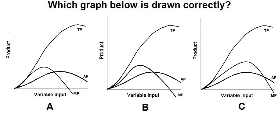
The costs curves show us how costs change with output. The production function in lesson 7a showed us how output changes when we add more resources. They are related. We studied the production function so that we could learn about (1) specialization and teamwork, (2) getting crowded, and (3) overcrowded, because these concepts will help us undersrand the shapes of the cost curves. Remember: whenever we learn a new graph we must understand it shape (For all graphs: DEFINE, DRAW, DESCRIBE SHAPE).

In this lesson we will be looking at the SHORT RUN GRAPHS, We studied the definition of "short run" in chapter 4b. It doesn't really have much to do with time. The short run in some industries is longer than the long run in other industries. In the short run the quantity of at least one resource is fixed -does not change. We will usually assume that the number of factories or the size of the factory does not change. So in the short run we are adding more resources to an EXISTING factory . . . and it may get crowded or overcrowded. We will look at the long run costs (when we can change the numberr of factories or the size of the factories) in the next lesson, 7c.

Finally, we will be looking at three types of costs: fixed, variable, and total (fixed plus variable), and three "families" of costs: total, average, and marginal. By the end of this lesson you should be able to and correctly Define, Draw, and Describe the shapes of: TFC, TVC, TC, AFC, AVC, ATC, and MC. (For all graphs: DEFINE, DRAW, DESCRIBE SHAPE).

Short Run Total Cost Graphs:

Short Run Average Cost Graphs:

Topics:

  • short run cost curves

Readings:

  • Ch. 7, pp. 140-152

Video Lectures: [Cengage login] [TW login] [notes]

  • 7.3-1 Defining Variable Costs [TW 4.2.1 (4:23)]
  • 7.3-2 Graphing Variable Costs [TW 4.2.2 (4:57)]
  • 7.3-3 Defining Marginal Costs [TW 4.3.1 (6:41)]
  • 7.3-4 Deriving the Marginal Cost Curve [TW4.3.2 (10:59)]
  • 7.3-5 Understanding the Mathematical Relationship between Marginal Cost and Marginal Product [TW 4.3.3 (10:26)]
  • 7.3-6 Defining Average Variable Costs [TW 4.4.1 (5:37)]
  • 7.3-7 Understanding the Relationship between Marginal Cost and Average Variable Cost [TW 4.4.3 (7:54)]
  • 7.3-8 Defining and Graphing Average Fixed Cost and Average Total Cost [TW 4.5.1 (6:55)]
  • 7.3-9 Calculating Average Total Cost [TW 4.5.2 (4:51)]
  • 7.3-10 Putting the Cost Curves Together [TW 4.5.3 (4:51)]
  • 7.3-11 Shifts in the Cost Curves [TW 4.6.4 (3:26)]

Optional Review Videos:

Discussion Questions:

  • Do the TC curve and TVC curve get closer together?
  • Do the ATC curve and AVC curve get closer together?
  • Where does the MC curve cross the ATC and the AVC curves?
  • What happens to TC when MC is declining? when MC is increasing?

Must Know / Outcomes:

  • Define and understand the terms and concepts listed at the end of the chapter.
  • Distinguish between fixed, variable and total costs
  • Explain the difference between average and marginal costs
  • Compute and graph AFC, AVC, ATC, and marginal cost when given total cost data
  • Explain how TC, TVC, and TFC relate to one another
    • do TC and TVC get closer together?
  • Explain how AVC, ATC, and MC relate to one another
    • do ATC and AVC get closer together?
    • why does MC cros ATC and AVC at their lowest points?
  • Explain the shapes of the total, average, and marginal cost curves (TC, TVC, TFC, ATC, AVC, AFC, and MC)
  • Relate average product to average variable cost, and marginal product to marginal cost
  • Explain what happens to the cost curves if there is a change in fixed costs; variable costs (what can cause cost curves to rise or fall?)

WHY?


7c   Production Costs in the Long Run

Be sure that you can define "short run" and "long run" (see chapter 4). Note that in the next unit we will always use long run graphs to find the allocatively and productively efficient quantities.

As always, be sure you know why the long run ATC curve has the shape it does; For all graphs: DEFINE, DRAW, DESCRIBE SHAPE.

Topics:

  • short run cost curves continued
  • long run costs

Readings:

  • Ch 7, 152-162

Video Lectures: [Cengage login] [TW login] [notes]

  • SHORT RUN COSTS [continued]
  • PRODUCTION AND COSTS IN THE LONG RUN
    • 7,4-1 Defining the Long Run [TW4.6.1 (5:55)]
    • 7.4-2 Determining the Firm's Return to Scale [TW 4.6.2 (9:01)]
    • 7.4-3 Understanding the Short Run and Long Run Average Cost Curves [TW 4.6.3 (15:06)]

Discussion Question:

  • Why are there many hardware stores in Illinois but only three automobile production plants?

Must Know / Outcomes:

  • Define and understand the terms and concepts listed at the end of the chapter.
  • Explain the difference between short run and long run costs
  • State why the long run average cost is expected to be U shaped
  • List and explain the causes of economies and diseconomies of scale
  • Indicate the relationship between economies of scale and number of firms in an industry and their sizes


Unit 3: PRODUCT MARKETS and EFFICIENCY

8/9a   Pure Competition - Characteristics and Short Run Equilibrium

In chapters 8, 9, 10, and 11 we will be looking the producer decision of HOW MUCH TO PRODUCE. We will use benefit cost analysis (MB=MC) to find the profit maximizing quantity or WHAT WE GET. Once we know how much businesses will produce, we will ask: Is this quantity efficient (both allocatively and productively) or WHAT WE WANT?

We already know that businesses will maximize profits when they produce the equilibrium quantity (chapter 3). We also know that for competitive markets this will be the efficient quantity (except in a few situations where the market fails - chapter 5).

We will begin by looking at competitive markets in chapters 8 and 9. We should not be surprised that when competitive markets produce the profit maximizing quantity, they will also be producing the allocatively and productively efficient quantities.

For each of the four product market models (chapters 8-11) you should use the following general outline to guide your studying:

General Outline for Each Model:
  1. Know the model's characteristics and examples (See the "Ch. 8 - 4 PRODUCT MARKET MODEL" quiz on our Blackboard site.)
  2. Be able to explain the shape of the demand curve
  3. Draw the short run equilibrium graphs for (a) profit maximizing firms, (b) loss minimizing firms, and (c) firms that will shut down
  4. Draw the long run equilibrium graph and find the profit maximizing quantity (WHAT WE GET), allocatively efficient quantity (WHAT WE WANT), and the productively efficient quantity. (See the 3 Rules and 4 Models Yellow Pages.)
  5. Understand any other issues associated with the model

Never forget this: To maximize profits business will produce the quantity where MR=MC.

Topics:

  • market structures
  • pure comp. - short run equilibrium

Readings:

  • Ch. 8 ALL

Video Lectures: [Cengage login] [TW login] [notes]

  • MARKET STRUCTURE
    • 10.1-1 Understanding Market Structure [TW 5.1.3 (10:55)]
  • WHAT IS A PERFECTLY COMPETITIVE MARKET? (PURE COMPETITION)
    • 8.1-1 Understanding the Role of Price [TW 5.1.2 (3:43)]
    • 8.2-1 Calculating Total Revenue [TW 5.1.1 (3:36)]
  • PURE COMPETITION - SHORT RUN PROFIT MAXIMIZATION
    • 8.3-1 Finding the Firm's Profit Maximizing Output Level [TW 5.2.1 (14:24)]
    • 8.3-2 Proving the Profit Maximizing Rule [TW 5.2.2 (4:20)]
    • 8.3-3 Calculating Profit [TW 5.2.3 (12:26)]
    • 8.3-4 Calculating Loss [TW 5.2.4 (9:13)]
    • 8.4-1 Finding the Firm's Shut-Down Point [TW5.2.5 (8:35)]
  • PURE COMPETITION - SHORT AND LONG RUN MARKET SUPPLY
    • 8.5-1 Deriving the Short-Run Market Supply [TW 5.3.1 (20:44)]
    • 8.7-1 Deriving the Long-Run Market Supply Curve [TW 5.3.4 (9:13)]

Discussion Questions:

  • Why is the demand curve horizontal (perfectly price elastic) for purely competitive firms?
  • If MR = MC, what will a firm's profits be?

Must Know / Outcomes:

  • Define and understand the terms and concepts listed at the end of the chapter
  • List the four basic market models and characteristics of each.
  • Describe characteristics of a purely competitive firm and industry.
  • Explain how a purely competitive firm views demand for its product and marginal revenue from each additional unit sale.
  • Compute and graph average, total, and marginal revenue when given a demand schedule for a purely competitive firm.
  • Use both total revenue minus total-cost and marginal revenue = marginal cost approaches to determine short run price and output that maximizes profits (or minimizes losses) for a competitive firm.
    • with a table of data
    • on a graph with numbers
    • on a graph using geometry (graph with letters)
  • Find the short run supply curve when given short run cost schedules for a competitive firm.


8/9b   Pure Competition - Long Run Equilibrium and Efficiency

 Again, we return to the central issue of economics: reducing scarcity (the 5Es). In chapters 9, 10, and 11 we will see if industries are (1) allocatively efficient, and (2) productively efficient, in the long run.

This would be a good time to review the 5Es online reading from lesson 1b and reacquaint yourself with the definitions and examples of allocative and productive efficiency. Allocative efficiency means producing the mix of goods and services that maximize society's satisfaction and productive efficiency means producing at a minimum cost.

What else do we know? In chapter 1 we learned about benefit-cost analysis (marginal analysis). From chapters 3 and 5 we know that we find the allocatively efficient quantity where MSB = MSC and where consumer plus producer surplus are maximized. In chapter 4 we learned the definitions of short run and long run.

In chapters 9, 10, and 11 we will put all of this together to see if businesses are efficient. Of course we do not have time to study every individual business or industry, so we will exame the efficiency of four groups of industries or the four product market models.

In chapter 2 we learned that competitive markets are efficient. In chapter 8 we learned the characteristics of comptitive markets and how competitive businesses find the profit maximizing quantity to produce (where MR=MC or WHAT WE GET). Here, we will learn that since there are no barriers to entry in the long run the competitive markets will produce

Never forget this: To maximize profits business will produce the quantity where MR=MC.

Topics:

  • pure comp - long run equilibrium
  • pure comp and efficiency
  • marginal coat pricing

Readings:

  • Ch. 9, ALL

Video Lectures: [Cengage login] [TW login] [notes]

Discussion Questions:

  • How do you find the profit maximizing quantity?
  • How do you find the alocatively efficient quantity?
  • How do you find the productively efficient quantity?
  • Why does a purely competitve firm earn zero economic profits (normal profits) in the long run?

Must Know / Outcomes:

  • Define and understand the terms and concepts listed at the end of the chapter
  • Distinguish between the short run and the long run in pure competition.
  • Explain the long run equilibrium position for a competitive firm using entry and exit of firms to explain adjustments from nonequilibrium positions.
  • Describe the role of profits and losses in achieving the long run equilibrium
  • Explain the shape of long run industry supply curves in constant cost and increasing cost industries.
  • Differentiate between productive and allocative efficiency.
  • Explain why allocative efficiency and productive efficiency are achieved where P = minimum ATC = MC.
  • Explain why allocative efficiency and productive efficiency are consistent with maximizing consumer and producer surplus and an efficient use of resources.
  • Evaluate the impact of creative destruction on purely competitive industries


10/18a  Monopoly: Charcteristics and Short-Run Equilibrium


Topics:

  • monopoly - short run equilibrium

Readings:

  • Ch. 10, pp. 194-203

Video Lectures: [Cengage login] [TW login] [notes]

  • MONOPOLY
    • 9.1-1 Defining Market Power [TW 6.1.1 (10:10)
    • 9.2-1 Defining Marginal Revenue for a Firm with Market Power [TW 6.1.2 (12:43)]
  • PROFIT MAXIMIZATION FOR A MONOPOLY
    • 9.3-1 Determining the Monopolist's Profit Maximizing Output and Price [TW 6.1.3 (14:18)]
    • 9.3-2 Calculating a Monopolist's Profit and Loss [TW 6.1.4 (6:24)]
  • OPTIONAL

Discussion Questions:

  • Why is the demand curve for a monopoly downward sloping?
  • Why is the MR curve below the demand curve?
    OR:
    Why is the extra revenue that a monopoly receives from selling one more unit (MR) less than the price that they charge for that unit (D)?

Must Know / Outcomes:

  • Define and understand the terms and concepts listed at the end of the chapter
  • List the five characteristics of pure monopoly.
  • Explain the difference between a "pure" monopoly and a "near" monopoly.
  • List and give examples of the four barriers to entry.
  • Describe the demand curve facing a pure monopoly and how it differs from that facing a firm in a purely competitive market.
  • Compute marginal revenue when given a monopoly demand schedule.
  • Explain why the marginal revenue is equal to the price in pure competition but not in monopoly.
  • Determine the price and output level the monopoly will choose given demand and cost information in both table and graphic form.


10/18b Monopoly: Long-Run, Efficiency, and Regulation


Topics:

Monopoly

  • Long Run Equilibrium
  • Efficiency
  • Price Discrimination
  • Natural Monopolies and Regulation

Readings:

  • Ch 10, pp, 203-214
  • Chapter 18:
    • pp. 376-382 Antittrust Policy: Issues and Impacts
    • pp. 381-383 Industrial Regulation
    • pp. 383-384 Deregulation

Video Lectures: [Cengage login] [TW login] [notes]

Discussion Questions:

  • Why does a monopoly earn economic profits in the long run?
  • We know that single price monopolies are allocatively inefficient in the long run. What happens to allocative efficiency if the monopoly can price discriminate?
  • Why does the Illinois government allow ComEd to have a monoply on the distribution of electricity in northern Illinois?

Must Know / Outcomes:

  • Discuss the economic effects of pure monopoly on price, quantity of product produced, allocative and productive efficiency, distribution of income, and technological progress.
  • Give examples of how new technology has lessened monopoly power.
  • Define price discrimination, list three conditions necessary for price discrimination, explain how price discrimination affects allocative efficiency, explain why profits and output will be higher for a discriminating monopoly.
  • Identify two pricing strategies of monopoly regulation and explain the dilemma the regulators face in utilizing these strategies
  • Explain why a regulated monopoly does not have an incentive to reduce costs.

11a Monopolistic Competition


Topics:

  • monopolistic competition

Readings:

  • Ch. 11, pp. 216-223

Video Lectures: [Cengage login] [TW login] [notes]

  • MONOPOLISTIC COMPETITION
    • 10.1-2 Defining Monopolistic Competition [TW 6.4.1 (7:01)]
    • 10.2-1 Short-Run Profit Maximization for a Monopolistically Competitive Firm - Understanding Pricing and Output in Monopolistic Competition [TW 6.4.2 (8:58)]
    • Monopolistic Competition (econclassroom.com 20:51 -- efficiency begins at 15:00 )
    • Monopolistic Competition in the Long-Run: Econ Concepts in 60 Seconds with AP Economics Teacher (ACDCEcon 3:25)
      http://www.youtube.com/watch?v=erdzOu3juNI

Discussion Questions:

  • Why does a monopolistically competitive firm earn zero economic profits (normal profits) in the long run?
  • Are monopolistically competitive firms inefficient?

Must Know / Outcomes:

  • Define and understand the terms and concepts listed at the end of the chapter
  • List the characteristics of monopolistic competition.
  • Explain how product differentiation occurs in similar products.
  • Determine the profit maximizing price and output level for a monopolistic competitor in the short run when given cost and demand data.
  • Explain why a monopolistic competitor will realize only normal profit in the long run.
  • Identify the reasons for excess capacity in monopolistic competition.
  • Explain how product differentiation may offset these inefficiencies.


11b Oligopoly


Topics:

  • oligopoly
  • mergers

Readings:

  • Ch. 11, pp. 223-240
  • Ch 11 appendix, pp. 241-244
  • Ch. 18 Mergers, pp. 379-380

Video Lectures: [Cengage login] [TW login] [notes]

Discussion Questions:

Must Know / Outcomes:

  • Define and understand the terms and concepts listed at the end of the chapter
  • Describe the characteristics of an oligopolistic industry.
  • Differentiate between homogeneous and differentiated oligopolies.
  • Identify and explain the most important causes of oligopoly.
  • Describe and compare the concentration ratio and the Herfindahl index as ways to measure market dominance in an industry.
  • Distinguish between three types of mergers. (Ch. 18)
  • Explain how the Herfindahl index is used as a guideline by the government in deciding whether to permit horizontal mergers. (Ch. 18)
  • Use a profit-payoffs matrix (game theory) to explain the mutual interdependence of two rival firms and why oligopolists might tempt to cheat on a collusive agreement.
  • Identify three possible models of oligopolistic price-output behavior.
  • Use the kinked demand curve theory to explain why prices tend to be inflexible.
  • Explain the major advantages of collusion for oligopolistic producers.
  • List the obstacles to collusion behavior.
  • Explain price leadership as a form of tacit collusion.
  • Explain why oligopolies may prefer nonprice competition over price competition.
  • List the positive and negative effects of advertising.
  • Explain why some economists assert that oligopoly is less desirable than pure monopoly.
  • Explain the three ways that the power of oligopolists may be diminished.

Unit 4: RESOURCE MARKETS, INEQUALITY, and IMMIGRATION

12a Demand for Resources


Topics:

  • demand for resources

Readings:

  • Chapter 12:
    • pp. 248-257
    • pp. 260-261
  • DO NOT STUDY: "Optimal Combination of Resources", pp. 257-260

 Video Lectures: [Cengage login] [TW login] [notes]

Discussion Questions:

  • What is MRP=MRC?
  • What is W = VMP or W = (P x MP)?
  • What are the determinants of resource demand?
  • What are the determinants of the price elasticity of demand?

Must Know / Outcomes:

  • Present four major reasons for studying resource pricing.
  • Explain the concept of derived demand as it applies to resource demand.
  • Determine the marginal-revenue-product schedule for an input when given appropriate data.
  • State the principle employed by a profit maximizing firm in determining how much of a resource it will employ.
  • Apply the MRP = MRC principle to find the quantity of a resource a firm will employ when given the necessary data.
  • Explain why the MRP schedule of a resource is the firm's demand schedule for the resource in a purely competitive product market.
  • Explain why the resource demand curve is downward sloping when a firm is selling output in a purely competitive product market; an imperfectly competitive product market.
  • List the three determinants of demand for a resource and explain how a change in each of the determinants would affect the demand for the resource.
  • Explain what demand factors have influenced the growth and decline of the occupations listed in Tables 12.5 and 12.6.
  • List three determinants of the price elasticity of demand for a resource, and state how changes in each would affect the elasticity of demand for a resource.
  • Explain the marginal productivity theory of income distribution and present two criticisms of it.
  • Define and identify terms and concepts listed at the end of the chapter.

13a Wage Determination (Labor Markets)


 Topics:

  • wage determination

Readings:

Video Lectures: [Cengage login] [TW login] [notes]

Discussion Questions:

  • Explain, be sure to discuss price elasticity of demand for workers: " . . .if we woke up tomorrow and fast food restaurants had doubled worker pay tomorrow . . . I'm sure you would see a lot of jobs lost , . . . But that’s only part of the story, Baker argues. Even if there was, let’s say, a 20 or 30 percent drop in employment at these places (Saltsman told me he projects there could be up to a 27 percent drop), the remaining workers would still “take home twice as much pay. They're still way better off,” says Baker." From:
    http://www.marketplace.org/topics/wealth-poverty/fast-food-strike-walk-outs-and-drive-throughs

Must Know / Outcomes:

  • List those factors that have led to an increasing level of real wages in the U.S. historically.
  • Determine the equilibrium wage rate and employment level when given appropriate data for a firm operating in a:
    • purely competitive product and labor market;
    • a firm operating in a monopolistically competitive product market and a purely competitive labor market;
    • and a firm operating in a purely competitive product market and a monopsonistic labor market.
  • Illustrate graphically how wage rates are determined in purely competitive and monopsonistic labor markets.
  • List the methods used by labor organizations (labor unions) to increase wages and the impact each has on employment. Give specific examples.
  • Illustrate graphically how an inclusive (industrial) union and an exclusive (craft) union would affect wages and employment in a previously competitive labor market.
  • Explain and illustrate graphically wage determination in the bilateral monopoly model.
  • Present the major points in the cases for and against the minimum wage.
  • Explain the demand factors that create wage differentials.
  • Explain the supply factors that create wage differentials.
  • Describe briefly salary systems in which pay is linked to performance rather than to time.
  • Define and identify terms and concepts listed at the end of the chapter.

20a Income Inequality and Discrimination


Topics:

  • income inequality

Readings:

Video Lectures: [Cengage login] [TW login] [notes]

Discussion Questions:

Must Know / Outcomes:

  • Describe the distribution of income in the United States by personal income categories by households and quintile distribution by households.
  • Explain how a Lorenz curve is used to describe income inequality.
  • Explain how a Gini ratio measures income inequality and is related to the Lorenz curve.
  • Discuss the impact of income mobility on income distribution data.
  • Explain the broadened concept of income, which includes the effects of taxes and transfer payments, and how this affects the extent of inequality of income and poverty in the U.S.
  • List seven causes of an unequal income distribution.
  • Describe changes and causes for the changes in inequality since 1970.
  • State and evaluate the cases for and against income inequality, using the equality vs. efficiency argument ["The Case for Equality: Maximizing Total Utility = The President Obama Example (fig. 20.3)]
  • Occupational Discrimination - The Crowding Model - The Model (figure 20.7)


 22a Immigration


Topics:

  • Immigration

Readings:

Video Lectures: [Cengage login] [TW login] [notes]

Discussion Questions:

Must Know / Outcomes:

  • Understand the historical pattern of legal and illegal immigration the United States.
  • Understand what motivates an individual to migrate.
  • List the factors influencing the decision to migrate.
  • Understand the potential impact immigration can have on wage rates, efficiency, and output. "Impact on Wage Rates, Efficiency, and Output" (Figure 22.3)
  • Understand how immigration can affect income shares.
  • Identify potential complications with the traditional model of immigration: Remittances, Full-Employment or Unemployment, and Complements and Substitutes.
  • Understand the effect immigration to the United States has on Federal, State, and Local governments' fiscal position.
  • Understand the illegal immigration debate in the context of job "crowding-out. ["Impact of Illegal Workers in a Low Wage Labor Market"]
  • Explain the potential price effects that illegal immigration can have on an economy.
  • Understand the concept of 'optimal' immigration.