 |
- Multiplier example: see fpexample.htm
- REVIEW MULTIPLIERS
- The MULTIPLIER in the NEWS
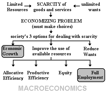
The issues discussed in macroeconomics are:
1. full employment
2. price stability
3. economic growth
In the 5Es lesson we have already discussed the importance of these topics in reducing scarcity and receiving the maximum satisfaction possible from our limited resources.
 |
Here we will look at fiscal policy designed to achieve low unemployment or low inflation.
The following is from the lecture on Macroeconomic Policies
(NOTE: when I use the term "policies", I always mean "government policies").
What is the role of the government in a market economy? In a market economy (capitalist economy) the government has a limited role, but some people believe that the government should try to help the economy maintain full employment and low inflation. We have discussed in the 5 Es lesson that unemployment results in greater scarcity since some resources are not being used so less will be produced. Government policies may be able to help the economy achieve full employment and therefore reduce scarcity.
Stabilization Policies
Definition: government policies design to reduce UE and/or inflation All the policies discussed here can be classified as stabilization policies.There are two major types of stabilization policies:
- demand-management policies
- supply-side policies
Demand-Management Policies
Definition: Policies design to shift the AD curve in order to reduce unemployment or to reduce inflation.Tools -- Some of the determinants of AD can be manipulated by the government to achieve these goals.
There are two types of demand-management policies depending upon WHO conducts the policy:
- fiscal policy is undertaken by the president and the congress, and
- monetary policy is undertaken by the Federal Reserve Board (often called the "fed").
Fiscal Policy
Definition: discretionary fiscal policyDeliberate changes in taxes (tax rates) and government spending by Congress to promote full-employment, price stability, and economic growth.Fiscal Policy tools
a. government purchases (spending)
b. taxes
c. bothExpansionary Fiscal Policy
- An increase in government expenditures for goods and services,
- a decrease in taxes,
- or some combination of the two
- for the purpose of increasing aggregate demand and expanding real output
- this will reduce UE
The goal of expansionary fiscal policy is to reduce unemployment. Therefore the tools would be an increase in government spending and/or a decrease in taxes. This would shift the AD curve to the right increasing real GDP and decreasing unemployment, but it may also cause some inflation.
Contractionary Fiscal Policy
- A decrease in government expenditures for goods and services,
- an increase in net taxes,
- or some combination of the two
- for the purpose of decreasing aggregate demand and thus controlling inflation.
The goal of contractionary fiscal policy is to reduce inflation. Therefore the tools would be an decrease in government spending and/or an increase in taxes. This would shift the AD curve to the left decreasing inflation, but it may also cause some unemployment.
FISCAL POLICY WE ALREADY KNOW:
If there is UE?
- increase G
- decrease T
- both
If there is IN?
- decrease G
- increase T
- both
NOW WE ARE GOING TO LEARN:

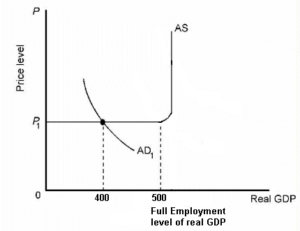
So we already know that if there is unemployment the appropriate fiscal policy would be to increase government spending and/or decrease taxes. Here we will discuss HOW MUCH should government spending be increased or taxes cut?
GDP = C + I + G + Xn 400 Look at the graph to the right and the formula above. You
can see that this economy is at equilibrium producing an
output of $400, but if there were full employment, a real
GDP of $500 could be achieved. Therefore, this economy has
an unemployment problem and is not producing as much as it
could. What is the appropriate fiscal policy could the
government use to move this economy to full employment?
We know that the government could increase government spending
and/or reduce taxes to increase AD and achieve full employment. Here,
let's just concentrate on government spending.
By HOW MUCH should government spending be increased to achieve and equilibrium of $500 and full employment?
|
GDP |
= |
C |
+ |
I |
+ |
G |
+ |
Xn |
|
to $100 |
? |
One would think that if government spending was increased by $100 that GDP would go up by $100, BUT THIS IS NOT THE CASE! What we are going to learn in this chapter is that a small initial increase in spending results in a much larger change in GDP. This is called the MULTIPLIER EFFECT. A small initial change in spending will result in a larger change in GDP as the spending change works it way through the economy.
How the multiplier process works:
This is because an initial change in spending will cause an initial increase in GDP and it also becomes income to someone else. (If I buy a new car, people who built and sold that car earn income equal to the price of the car.) What will these people do with their additional income? Well, they will spend some and save some. The amount that they spend increases GDP even more AND it also becomes income to someone else. These other people will spend some of this additional income and save some. The amount THEY spend increases GDP again and becomes income to someone else. This process continues so that the TOTAL change in GDP is much larger than the initial change in spending.
This multiplier process helps explain why cities want the superbowl, political conventions, or the Olympics to be held in their town. It's not just because these activities bring in people who will spend money and create jobs, but more importantly, this initial change in spending begins the multiplier process so that the total economic effect and the number of jobs created is much larger than the initial spending on these activities alone would cause.
Read this article from the Philadelphia Inquirer newspaper (http://home.phillynews.com/gop/news/impa110698.asp). the Republican National Convention was held in Philadelphia in 2000 and in San Diego in 1996. It is clear that civic leaders understand the multiplier effect when they discuss "spinoff benefits".
------------- ------------------ --------------------- ------------------ --------------------- ---------
The Philadelphia Inquirer, November 6, 1998
Plentiful gains seen from GOP
The publicity for the city may be priceless. The visitors' spending could reach $300 million.
By Howard Goodman
INQUIRER STAFF WRITER
When the elephants thunder into Philadelphia in 2000, the vibrations are expected to shake an incredibly bountiful money tree, showering dollars all over the region.
The economic impact of the Republican National Convention will almost certainly exceed $125 million in direct spending on hotel rooms, meals and the like, along with at least $175 million in spinoff benefits (emphasis added), David L. Cohen said yesterday. Cohen, Mayor Rendell's former chief of staff, is cochairman of Philadelphia 2000, the committee formed to woo a political convention.
The estimate is based on a Federal Reserve Board study of the economic blessings felt in Chicago from the 1996 Democratic convention, with a little extra figured in for four years' worth of inflation, Cohen said.
"There is no convention you can host that has a greater economic impact than a national political convention," he said. "Most people agree the only thing you can host that has a greater economic impact is the Olympics."
. . . . .In San Diego, where the Republicans last met, business leaders still bask in the 1996 convention's glow. "We look at the convention as a weeklong television commercial for your city as a destination," Salvatore Giametta, a spokesman for the San Diego Convention and Visitors Bureau, said in an interview this summer.
. . . . .
According to the Greater San Diego Area Chamber of Commerce, the four-day convention attracted 30,000 visitors who spent $26 million on hotel rooms. But there has been no follow-up study to show the convention's broader effect on the San Diego economy.
Despite the lack of data, San Diego "absolutely" would host a convention again, Giametta said. "We think it was good for the tourism industry without a doubt."
Brian Ford, an accountant for Philadelphia 2000, said that insisting on a study to prove that Philadelphia will benefit mightily from the GOP meeting "is like saying you need a study to show that a car works.". . . . .
Above we said that the multiplier works "because an initial change in spending will cause an initial increase in GDP and it also becomes income to someone else. (If I buy a new car, people who built and sold that car earn income equal to the price of the car.) What will these people do with their additional income? Well, they will spend some and save some. The amount that they spend increases GDP even more AND it also becomes income to someone else." This process then goes on and on . . . but why does it eventually stop or does it go on forever? If you reread the explanation of the multiplier process above you will get a clue as to why the process eventually stops. Notice that we said "What will these people do with their new income? Well, they will spend some and save some." People do not spend 100% of any additional income that they receive. the spend some and SAVE SOME. So that the additional spending is less than their increase in income. And when this additional spending becomes income to someone else, they sill save some and spend even a smaller amount. This will continue until the total change in savings is equal to the initial increase in spending. When this occurs there is nothing left to spend and the process stops.
To understand the multiplier process we must gain a better understanding of how consumption and saving respond to changes in income. the table below is for a hypothetical economy. All values are in $ billions.
$ 0 $ 40 100 120 200 200 300 280 400 360 500 440
As expected as the economy's GDP (income) increases, household
consumption increases. GDP and consumption are directly related. If
we graphed this consumption data we would get:
(income)
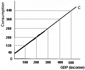
Notice that when income is equal to $ 0, there is still some consumption ($ 40 billion). this is called "autonomous consumption". It is consumption that is not related to income. Think about what a GDP of $ 0 represents. If GDP, or an economy's income, were equal to $0, this means that nothing was produced in this. If an economy does not produce a thing, would there still be some consumption? Yes, but how? they would consume goods that were saved from earlier periods. Of course, a GDP of $0 is a ridiculous concept, but there are two components to household consumption: (1) autonomous consumption that is not related to income, and (2) induced consumption or consumption that is directly related to income.
Now, to understand,a and calculate, the multiplier, we need to complete the table.
First we need some simplifying assumptions to make our model easier to understand:
|
GDP |
= |
C |
+ |
I |
Given these assumptions we can calculate savings (S). With these assumptions there are only two things that consumers can do with their income, spend it (C) or save it (S). So:
|
income |
= |
C |
+ |
S |
Therefore, we can calculate savings:
$ 0 $ 40 $ - 40 100 120 - 20 200 200 0 300 280 20 400 360 40 500 440 60
Notice that savings is directly related to income. When income
increases both consumption and savings increase.
(income)
Average Propensity to Consume (APC) and Average Propensity to Save (APS)
With this data we can calculate the APC and APS for each level of income.
APC is the fraction of the economy's total income that is spent (consumed) and APS is the fraction of total income that is saved.
|
|
|
|
APC = |
-------- |
|
income |
|
|
|
|
APS = |
-------- |
|
income |
When we calculate APC and APS we get:
$ 0 $ 40 $
- 40 100 120 - 20 1.2 - 0.2 200 200 0 1.0 0 300 280 20 0.93 .07 400 360 40 0.90 .10 500 440 60 0.88 .12
(income)
Notice that for each level of income: APC + APS = 1. Given our assumptions there are only two things that consumers can do with their income spend it or save it. If you add the fraction of the total income that is spent (APC) and the fraction of the total income that is saved (APS) we get all of our income, or 1.
Can you think of anything else that we can do with our income besides spend it or save it? Many students will answer "invest it". But what does investment mean in economics? Investment is the accumulation of capital. "Capital" is a manufactured resource. Therefore, "investment" occurs when a carpenter buys a hammer or if McDonald's builds a new restaurant. Putting money into the stock market is NOT investment, it is savings.
Marginal Propensity to Consume (MPC) and Marginal Propensity to Save (MPS)
To understand the multiplier effect we need to know what happens to ADDITIONAL, or MARGINAL, income.
Earlier we explained that the multiplier works "because an initial change in spending will cause an initial increase in GDP and it also becomes income to someone else. (If I buy a new car, people who built and sold that car earn income equal to the price of the car.) What will these people do with their additional income?
With our consumption and savings data we can calculate the MPC and MPS for each level of income.
MPC is the fraction of the economy's additional income that is spent (consumed) and APS is the fraction of additional income that is saved.
"Marginal" means "additional" or "extra"
|
change in C |
|
|
MPC = |
----------------- |
|
change in income |
|
change in S |
|
|
MPS = |
----------------- |
|
change in income |
To calculate MPC and MPS select two levels of GDP or income. for example if income increases from $0 to $100, then consumption increases from $40 to 120. Therefore if income increases from $0 to $100 then the change in income is $100 and the change in consumption is $80. MPC is then equal to 0.8.
|
|
|
||||
|
MPC = |
--------------- |
|
|
|
|
|
|
|
If you do the same thing for MPS you will get MPS = 0.2.
$ 0 $ 40 $
- 40 100 120 - 20 1.2 - 0.2 0.8 0.2 200 200 0 1.0 0 0.8 0.2 300 280 20 0.93 .07 0.8 0.2 400 360 40 0.90 .10 0.8 0.2 500 440 60 0.88 .12 0.8 0.2
Notice that for each level of income, MPC + MPS = 1. There are
two things that you can do with additional income: spend a fraction
(MPC) and save a fraction (MPS). If you add these fractions together
you will get 1.
(income)
If you remember your 8th grade math you would recognize that our formula for MPC is actually the slope of the consumption graph.
|
|
|
||||
|
MPC = |
--------------- |
|
|
|
|
|
|
|
|
|
|
And the same is true for MPS:
|
|
|
One last item needs to be discussed: are MPC and MPS really constant? Note that in our table MPS equals 0.8 for all income levels and MPS equals 0.2. This means that if you get a raise (or additional income) of $1000 you would spend $800 of the raise (0.8 x 1000 = $800) and you would save $200 of it (0.2 x $1000 = $200). But is the fraction of additional income that is spent and saved really constant for all levels of income?
Let's assume that I am going to give two families $10,000 in additional income. So I go to the housing projects in Chicago and find a poor family and give them $10,000 and I fly to the state of Washington and find Bill Gates (probably the richest person in the world) and give him $10,000. Would they both spend and save the same fraction of this additional income?
No, the poor family would most likely spend the whole $10,000 and Bill Gates would probably spend nothing of the addition income. So the MPC of the poor family would be very high, or equal to 1, and the MPC of Bill Gates would be very low, or equal to 0. So as GDP or income increases, MPC should get smaller, or decrease, and MPS increases. This means the slope of the consumption graph should get smaller (flattens out) as GDP increases.
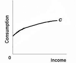
We will assume that the MPC is constant in this course. that way we can use straight line consumption graphs and we can find the MPC by finding its slope.
Given our simplifying assumptions we have an economy with only consumers and businesses. Therefore:
GDP = C + I
Now let's assume that in this economy (let's say that it represents the Chicago area) a new stadium worth $20 million is built. What is the total impact of this investment on the economy?
Well, if GDP is the total market value of all final goods and
services produced in an economy in one year , then building this $20
million stadium will increase GDP initially by $20.
GDP = Income = C + I + 20 + 20
![]()
But when $20 is spent (and therefore $20 is produced) $20 is also earned as income to those who did the producing. so income also increases by $20. What do these people do with this additional income? Well, they spend a part and save a part. How much do they spend and save? What concept tells us the change in consumption that results from additional income? . . MPC !
|
|
|
|
MPC = |
--------------- |
|
|
So if incomes go up by $20, consumption will increase by $16
Change in C = (MPC) x (change in income)
Change in C = (0.8) x ($20) = $16
and the change in S = $4
Change in S = (MPS) x (change in income)
Change in S = (0.2) x ($20) = $4
So we get the following
GDP = Income = C + I + 20 + 20 + 16 +16
![]()
![]()
![]()
And GDP has gone up by an additional $16, but so has income. What will they do with this income? They will spend 80% (MPC=0.8) of it and save 20% (MPS=0.2).
So we get the following:
GDP = Income = C + I + 20 + 20 + 16 +16 + 4 + 12.8 + 12.8 + 3.2
![]()
![]()
![]()
![]()
![]()
And GDP has increased by $12.8 and so has income, part of which will be spent and part saved. So consumption and GDP increase by $10.24 (0.8 x 12.8) and saving increases by 2.56 (0.2 x 12.8).
GDP = Income = C + I + 20 + 20 + 16 +16 + 4 + 12.8 + 12.8 + 3.2 + 10.24 + 10.24 + 2.56
![]()
![]()
![]()
![]()
![]()
![]()
![]()
This process will go on and on. When will it stop? If we add up all that has been saved and it equals 20, ( 4 + 3.2 + 2.56 + ...+...+...+...= 20) then there is nothing left to spend and the process stops. If you do this you will get the following total changes:
GDP = Income = C + I + 20 + 20 + 16 +16 + 4 + 12.8 + 12.8 + 3.2 + 10.24 + 10.24 + 2.56 total change total change total change + 100 + 80 + 20 + 20
![]()
![]()
![]()
![]()
![]()
![]()
![]()
![]()
![]()
![]()
![]()
So with an initial increase in spending of $20, GDP increases by $100.
The most important formula for you to learn is:
|
change in GDP |
= |
initial change in spending |
|
multiplier |
So using our data we get:
change in GDP initial change in spending multiplier
Graphically -- how does the multiplier work?
a. THIS IS IMPORTANT!
(Be sure you understand table 9-3 and Figure 9.8)b. $20 billion bill example (KNOW THIS!)
Assume: MPC = .8, and I increases by $20 billionc. the multiplier and the AS/AD graph: $20 billion bill in class example: See explanation below
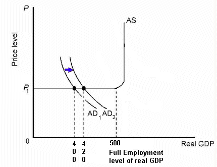
FROM TEXTBOOK (12.1)
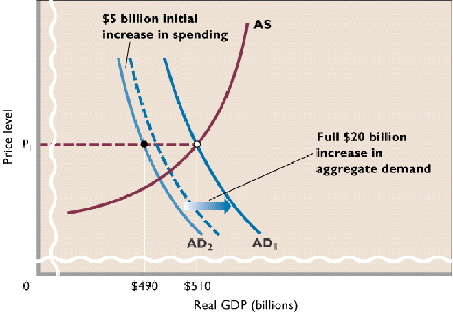
To see the multiplier in reverse read: : artbuchwaldmultiplier.htm
multiplier and marginal propensities (slopes)
a.
1
a. multiplier =
-------
MPS
b.
1
b. multiplier =
------------
1 - MPC
c. a larger MPC (or smaller MPS) has a larger multiplier
Now let's add government to our model.
GDP = C + I + G
Use these graphs to answer the questions that follow
|
|
|
ANSWERS:
1.
0.8
2.
0.2
3.
$400
4.
$500
OPTIONAL: Marginal Propensities to Consume and to Save
The Government Expenditures Multiplier
We know that a small initial change in spending will result in a multiplied effect on total spending in the economy, or:
change in GDP
=
initial change in spending
x multiplier
So to answer question # 5 above we have:
change in GDP
=
initial change in spending
x multiplier
+ $100
=
increase G by ?
x ?
If we knew what the multiplier was, we could easily calculate the change in government spending needed to increase GDP by $100 and achieve full employment.
1 1 multiplier =
-------- or ----------
MPS 1 - MPC
So:
1 1 multiplier =
-------- = ---------- =
5
MPS 0.2
And:
change in GDP
=
initial change in spending
x multiplier
+ $100
=
increase G by ?
x 5
and the increase in government spending needed to increase GDP by $100, and therefore achieve full employment, is $20.
change in GDP
=
initial change in spending
x multiplier
+ $100
=
increase G by 20
x 5 + $100
=
20
x 5
The Multiplier and Marginal Propensities
Notice that the size of the multiplier is inversely related to the size of the MPS. If the MPS is larger, the multiplier is smaller. This should make sense to you if you recall how the multiplier works. We said: "an initial change in spending will cause an initial increase in GDP and it also becomes income to someone else. (If I buy a new car, people who built and sold that car earn income equal to the price of the car.) What will these people do with their additional income? Well, they will spend some and save some. The amount that they spend increases GDP even more AND it also becomes income to someone else." So. if the MPS is larger (and the MPC is smaller) then the amount of additional income that is spent will be smaller and this will cause a smaller increase in GDP and a smaller increase in income to somebody else. Any time that more is saved and less is spent, GDP goes up by less.
You may want to try different MPC's and MPS's and see if this is true using the formulas below:
1 1 multiplier =
-------- or ---------- MPS 1 - MPC
The Multiplier Graphically
How does the multiplier effect look on our AS-AD graph? Here is our initial graph:

|
When spending (G) initially increases by $20 AD shifts to the right $20. |
|
|
Then income increases by $20 and we get $16 in induced consumption. |
|
|
This increases income by an additional $16 which increase induced consumption by $12.8 and so on until savings equals $20 and there is nothing left to spend. The total change in GDP equals $100. this is the initial $20 in government spending and a total of $80 in induced consumption. |
|
Review of Important Formulas
change in C
MPC =
-----------------
change in income
change in S
MPS =
-----------------
change in income
This is the central goal of this lesson. This is the concept that we are trying to understand!
change in GDP
=
(initial change in spending)
x (multiplier)
1 1 multiplier =
-------- or ---------- MPS 1 - MPC
The Lump-Sum Tax Multiplier
There are three fiscal policy tools:
Here, let's use the same data that we have been using to see by HOW MUCH taxes should be changed when using fiscal policy.
Use these graphs to answer the questions that follow
|
|
|
ANSWERS:
1.
0.8
2.
0.2
3.
$400
4.
$500
We know that a small initial change in spending will result in a multiplied effect on total spending in the economy, or:
change in GDP
=
change in taxes
x lump-sum tax multiplier
So to answer question # 5 above we have:
change in GDP
=
change in taxes
x lump-sum tax multiplier
+ $100
=
decrease T by ?
x ?
If we knew what the lump-sum tax multiplier was, we could easily calculate the change in taxes needed to increase GDP by $100 and achieve full employment.
First, what is a "lump-sum tax"?
To make things easier for us we will discuss "lump-sum taxes" rather then the much more common income tax. A lump-sum tax is a "tax per person" and it does not change with income. for example if the lump-sum tax was $500 per person I would have to pay $2000 for my family of four regardless of my income.
Next, we know that if taxes are cut, this will increase disposable income and therefore increase consumption:
The question we have here is HOW MUCH? Let's say they decrease taxes by $25. this then will increase disposable income (spendable income) by $25. If consumers have an additional $25 to spend consumption will go up by how much?
What tells us the change in consumption that results from a change
in income? . . . MPC!!!
If MPC = 0.8 then if disposable income increases by $25, consumption
will increase by $20
change in consumption = (0.8) x ($25)
change in consumption = $20
So what happens to GDP with the multiplier effect?
change in GDP
So when we cut taxes by $25, GDP increased by $100. What is the lump-sum tax multiplier?
|
|
|
|
|
|
|
|
|
|
|
|
|
|
|
|
|
|
So the lump sum tax multiplier is equal to -4.
There are two ways to calculate the lump-sum tax multiplier:
|
|
||
|
|
|
|
|
|
|
|
||||
|
|
|
|
|
|
|
|
and
The lump-sum tax multiplier is always negative and
ONE LESS THAN THE SIMPLE MULTIPLIER.
So in this example our simple multiplier is:
|
|
|
||||
|
multiplier = |
|
|
|
|
|
|
|
|
So the lump-sum tax multiplier is -4.
Fiscal Policy and the Balanced Budget Multiplier
There are three fiscal policy tools:
What happens if the government changes BOTH government spending AND taxes by the SAME AMOUNT And in the SAME DIRECTION?
We call this a "balanced-budget change". IT DOES NOT BALANCE THE FEDERAL BUDGET, but it doesn't make it any more unbalanced. If there is high unemployment and the government uses expasionary fiscal policy to try to reduce the unemployment they would increase government spending and/or decrease taxes. If they do this, spending goes up and tax revenues go down so this would lean to a budget deficit where they are spending more than they take in as taxes. Many people do not what the government to deficit spend.
So let's go back to our example and see what the government can do to reduce unemployment without creating a (larger) deficit. Use these graphs to answer the questions that follow.
|
|
|
ANSWERS:
1.
0.8
2.
0.2
3.
$400
4.
$500
So let's go back to our example and see what the government can do to reduce unemployment without creating a (larger) deficit. What balanced-budget change (changing both government spending and taxes by the same amount and in the same direction) could the government undertake to increase GDP in this economy by $100 and thereby achieve full employment?
(change G and T by
?)
What would happen if we increase G by $100 AND increase T by $100? If we increase G, this will increase GDP, but if we increase T, this will decrease GDP. If we do both, what happens?
.
.
.
It depends on HOW MUCH GDP changes.
So lets increase G and T both by $100. What happens?
Increase G by $100:
change in GDP = (initial change in spending) x (multiplier) + $500
=
increase G by 100
x 5 RESULT: GDP goes up by $500
Increase T by $100:
change in GDP = change in taxes x lump-sum tax multiplier - $400 = increase T by $100 x -4 RESULT: GDP goes down by $400
Back to our example: What balanced-budget change (changing both government spending and taxes by the same amount and in the same direction) could the government undertake to increase GDP in this economy by $100 and thereby achieve full employment?
So, if the government does both, GDP will go up by $500 and down
by $400 for a net change of
+ $100.
What is the balanced-budget multiplier?
(change G and T by
$100)
The balanced-budget multiplier is always a 1. This is because
the lump-sum tax multiplier is always one less than the simple (or
government spending) multiplier.
The Multiplier with Changes in the Price Level
We have been assuming that the price level does not change as AD increases (see graph).
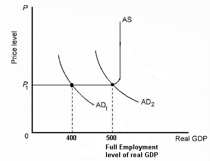
But in the real world as GDP increases and approaches the full employment level of output the price level will begin to rise and resource costs increase.
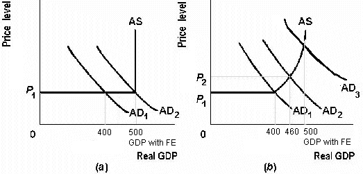
How does this inflation, which results from an increase in AD, affect the size of the multiplier? Or, what happens to the change in government spending needed to achieve full employment if we allow for inflation? Without inflation, and with an MPC of 0.8, if we increase government spending by $20 then GDP will increase by $100. the multiplier is 4. This will shift AD from AD1 to AD2 in both graphs above. In graph (a) without inflation the equilibrium GDP increases from $400 to $500. But in graph (b) with inflation the same horizontal shift in AD increases GDP from $400 to only $460. From the same change in government spending ($20) GDP increases a small amount. the multiplier is smaller.
To calculate the multiplier with changes in the price level you need to know the initial change in spending ($20 in our example) and the resulting total change in GDP ($60 from graph b above).
The Complex Multiplier
We have learned that in our simple model with no government, no inflation, and no foreign sector that the size of the multiplier is directly related to the MPC and inversely related to the MPS. In our simple model there are only two things that can be done with additional income: it can be spent or saved. the more that is NOT SPENT (saved) the smaller the change in GDP that results form a change in spending (i.e. the smaller the multiplier).
But in the real world there are more things to do with additional income than just spend it or SAVE it. You could also give it to the government as TAXES or spend it on IMPORTS. These last three are LEAKAGES from the income-expenditure stream which means they are income that we don't spend on our GDP so they don't generate additional income and contribute to the multiplier.
DI
C
AD
Leakages
Injections
S I T G M X
With more leakages, less additional spending is generated from an initial injection of spending, so the multiplier is smaller.
SIMPLE MULTIPLIER
1 simple multiplier =
-------- MPS COMPLEX MULTIPLIER
where MPS is the marginal propensity to save or the fraction of additional income that is saved
1 complex multiplier =
------------- MPS + MPT + MPM and MPT is the "marginal propensity to tax" or the fraction of additional income that is given to the government as taxes - this is very actually the marginal income tax rate
and MPM is the "marginal propensity to import" or the fraction of additional income that leaves the economy because it is spent on imports.
So in the real world there are more leakages from the income-expenditure stream and therefore the multiplier in the real-world is smaller than the simple multiplier that we will use most often in this class.
Outline:
Financing Deficits and the Multiplier1. borrowing
2. money creationDebt Retirement and the Multiplier
1. debt retirement
2. impounding
Definition: Discretionary Fiscal Policy
A deliberate changes in taxes (tax rates) and government spending by Congress to promote full-employment price stability and economic growth.
A. Discretionary Fiscal Policy and Multipliers
REVIEW MULTIPLIERS1.G and the multiplier
- we'll use the SIMPLE multiplier
- simple multiplier = 1/MPS
2.
T and the multiplier ( = multiplier - 1)
- we'll use the lump-sum tax multiplier
a. lump-sum tax
A tax which is a constant amount (the tax revenue of government is the same) at all levels of GDP.b. the lump-sum tax multiplier
1) is always one less than the simple multiplier, but negative2) lump-sum tax multiplier = -MPC / MPS
3.
G AND
T and the Multiplier
a.'s in G AND
's in T can be used in combination
b. "balanced budget" multiplier = 1
- what happens to the governments budget if they use expansionary FP?
- increase G
- decrease T
- What if the government changes both G and T by the same amount and in the same direction? Will GDP change?
- increase G increase GDP, but HOW MUCH?
- increase T decreases GDP, but HOW MUCH?
- The 'balanced budget multiplier" always has a value of 1 since the tax multiplier is always one less than the government spending multiplier
B. Expansionary Fiscal Policy (FP): Financing Deficits and the Multiplier
- expansionary FP leads to a greater government budget deficit
- how the government finances this deficit affect the size of the multiplier and the effectiveness of FP
1. borrowing
- If the government borrows to finance the deficit it may causes crowding out
Crowding-out Effect: A rise in interest rates caused by the Federal government’s increased borrowing in the money market and a resulting decrease in planned investment.
multiplier will be smaller
2. money creation
- If the Federal Reserve increases the MS at the same time:
(i.e. uses both expansionary FP and expansionary MP)This will keep interest rates down and reduce crowding out so closer to the simple multiplier
C. Contractionary Fiscal Policy: Debt Retirement and the Multiplier
- contractionary FP leads to a greater government budget surpluses
- how the government uses these surpluses affects the size of the multiplier and the effectiveness of FP
1. debt retirement
- If the government uses the surpluses to pay off some of its debt, this would cause interests rates to fall and increase AD
But the purpose of the contractionary FP was to fight inflation by decreasing AD
So debt retirement would make the contractionary FP less effective
a smaller multiplier
2. impounding
- If the governments impounds the surpluses - just keeps them
then the contractionary FP will be more effective
the multiplier will be closer to the simple multiplier
Non-discretionary Fiscal Policy: Built-in Stabilizers (pp. 248-253)
Outline:
What if the economy enters a recession and the government does NOTHING?Taxes are directly related to GDP (income) and Transfer Payments are indirectly related to GDP
Built-in Stabilizer
Tax Progressivity
Full-Employment Budget
A. When the economy enters a recession the government could:
- use expansionary FP (discretionary FP)
- do NOTHING (nondiscretionary FP)
B. What if the economy enters a recession and the government does NOTHING what happens?
- If Taxes are directly related to GDP (income),
- and Transfer Payments (welfare) are indirectly related to GDP,
- what happens to AD after entering a recession?
- taxes decrease
- government spending on welfare
- so AD increases even though the government did nothing
C. Built-in Stabilizer
A mechanism which increases government’s budget deficit (or reduces its surplus) during a recession and increases government’s budget surplus (or reduces its deficit) during inflation without any action by policy makers;the tax system is one such mechanism.
D. Tax Progressivity
A tax system wherein the average tax rate (tax revenue/GDP) rises with GDP.The more progressive the tax system, the greater the economy's built-in stability.
E. Full-Employment Budget
What happens to the government budget deficit if it uses expansionary FP?What happens to the government budget deficit if the economy enters a recession and the government does NOTHING?
So, if the government budget deficit increases when the economy enters a recession, does this indicate that the government is doing some SOMETHING (expansionary FP)?
Since deficits increase during recessions whether the government does SOMETHING or NOTHING we cannot use larger deficits as an indicator that the government is doing something.
Therefore, economists have created a the concept of a "full employment budget"
An increase in the full employment budget deficit is an indicator of discretionary expansionary FP
- actual budget
A listing of amounts spent by the Federal government (to purchase goods and services and for transfer payments) and the amounts of tax revenue collected by it in any (fiscal) year.- cyclical deficit
A Federal budget deficit which is caused by a recession and the consequent decline in tax revenues.- full-employment budget
A comparison of the government expenditures and tax collections which WOULD occur if the economy operated at full employment throughout the year.- structural deficit
The extent to which the Federal government’s expenditures exceed its tax revenues when the economy is at full employment (or the extent to which its current expenditures exceed the projected tax revenues which would accrue if the economy were at full employment); also known as a full-employment budget deficit.
Problems, Criticisms, and Complications (pp. 253-256)
Outline
Problems of Timing1. recognition lag
2. administrative lag
3. operational lagPolitical Problems
1. other goals
2. state and local finance
3. expansionary bias
4. a political business cycle?Crowding Out Effect
Fiscal Policy multiplier with inflation
A. Problems of Timing
1. RECOGNITION LAG is the elapsed time between the beginning of recession or inflation and awareness of this occurrence.2. ADMINISTRATIVE LAG is the difficulty in changing policy once the problem has been recognized.
3. OPERATIONAL LAG is the time elapsed between change in policy and its impact on the economy.
B. Political Considerations:
Government has other goals besides economic stability, and these may conflict with stabilization policy.1. A political business cycle may destabilize the economy:Election years have been characterized by more expansionary policies regardless of economic conditions. Some call this a political business cycle:The alleged tendency of Congress to destabilize the economy by reducing taxes and increasing government expenditures before elections and to raise taxes and lower expenditures after elections.
2. State and local finance policies may offset federal stabilization policies.
They are often procyclical, because balanced-budget requirements cause states and local governments to raise taxes in a recession or cut spending making the recession possibly worse.In an inflationary period, they may increase spending or cut taxes as their budgets head for surplus.
3. The crowding-out effect may be caused by fiscal policy.
a. REVIEW MULTIPLIERSb. DEFINITION: Crowding Out Effect
A rise in interest rates and a resulting decrease in planned investment caused by the Federal government’s increased borrowing in the money market.c. "Crowding-out" may occur with government deficit spending.
It may increase the interest rate and reduce private spending which weakens or cancels the stimulus of fiscal policy. (See Figure 12-5)
d. Some economists argue that little crowding out will occur during a recession.
e. Economists agree that government deficits should not occur at FE.,
f. it is also argued that monetary authorities could counteract the crowding-out by increasing the money supply to accommodate the expansionary fiscal policy.
4. Fiscal Policy multiplier with inflation
a. With an upward sloping AS curve, some portion of the potential impact of an expansionary fiscal policy on real output may be dissipated in the form of inflation.c. Graph
Fiscal Policy in the Open Economy (pp. 256-257)
Outline
Shocks Originating From AbroadNet Export Effect on the Multiplier
A. Shocks Originating From Abroad
Shocks or changes from abroad will cause changes in net exports which can shift aggregate demand leftward or rightward.B. Net Export Effect on the Multiplier
1. Definition:The idea that the impact of a change in monetary policy or fiscal policy will be strengthened or weakened by the consequent change in net exports;2. The net export effect reduces effectiveness of fiscal policy:
For example, expansionary fiscal policy may affect interest rates, which can cause the dollar to appreciate and exports to decline (or rise).3. Result:
- expansionary FP (goal: to increase AD and decrease UE), causes
- higher interest rates, which causes
- greater demand for the dollar by foreigners, which causes
- the dollar to appreciate, which causes
- US imports to increase and US exports to decrease, which
- decreases AD
- reduces the effectiveness of the exp. FP (small multiplier: REVIEW MULTIPLIERS)
Supply-Side Fiscal Policy and the Multiplier (pp. 257-258)
A. What is "Supply-Side FP" ?1. The contention that tax reductions will also shift the aggregate supply curve to the right.
(see the graph below).2. There are three main reasons for this:
a. Saving and investment -
- lower taxes will increase disposable incomes,
- thereby increasing household savings,
- lowering interest rates,
- and increase investment in new technology
- new technology increases productivity and,
- therefore shift aggregate supply to the right
b. Work incentives –
- lower tax rates will increase after tax wages from work,
- thereby increasing work incentives and productivity,
- therefore, shift aggregate supply to the right.,
c. Risk Taking –
- lower tax rates prod risk taking individuals and businesses to risk their energy and financial capital on new production methods and new products and,
- therefore, shift aggregate supply to the right.
B. Effect on the multiplier - REVIEW MULTIPLIERS
Larger multiplier: instead of going from Q1 to Q2 (simple multiplier) the economy goes to Q3C. Supply side economists sometimes argue that if lower taxes raise GDP, tax revenues may actually rise.
Laffer Curve
D. Many economists are skeptical of supply-side theories.
1. Effect of lower taxes on a supply is not supported by evidence.2. Tax impact on supply takes extended time, but demand impact is more immediate.