|
OPTIONAL:
- For table of the US Business cycle:
http://www.nber.org/cycles.html
- Here are examples of the types of news
articles that you should better understand
after completing this chapter: :
|
Introduction
Macroeconomics vs. Microeconomics
We have defined economics as the study of
how we choose to use limited resources to
obtain the maximum satisfaction of unlimited
human wants
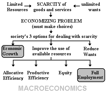
Macroeconomics Issues
The issues discussed in macroeconomics are:
1. full employment
2. price stability
3. economic growth
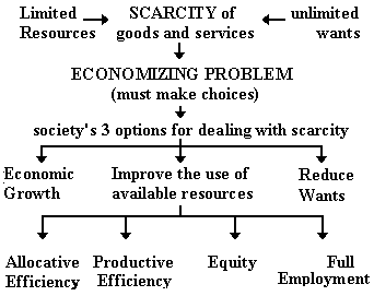
We have already discussed the importance of these topics
in reducing scarcity and receiving the maximum satisfaction
possible from our limited resources.
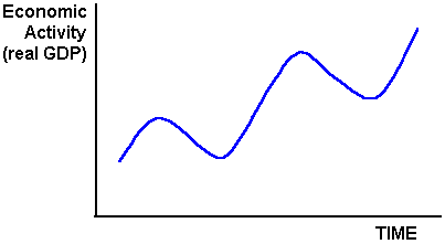
The Business Cycle
Over time the levels of unemployment (UE), inflation (IN)
and economic growth (EG) in an economy tend to fluctuate.
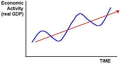
These fluctuations can be illustrated on a graph of the
business cycle.

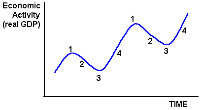
1. Economists have given terms to the four
phases of the business cycle:
a. #1 = peak
b. #2 = recession
c. #3 = trough
d. #4 = recovery

During each phase of the business cycle the
macroeconomic issues (UE, IN, and EG) change in a
particular way:
Peak:
During the peak of the business cycle economic
activity (output) is at its highest, therefore
unemployment is very low, but inflation is high.
Recession:
During the recession economic output declines ( a
recession is defined as six months of declining
output), therefore unemployment is rising and
inflation is declining.
Trough
During the trough economic output is is at its lowest,
therefore unemployment is at its highest and inflation
at its lowest.
Recovery:
During the recovery economic output increases,
therefore unemployment is declining and inflation is
rising.
The primary causes of the changes in output reflected
in the business cycle are changes in spending. This could
be changes in consumer spending (C), government spending
(G), business spending on new capital (I), or purchases
by foreigners Xn).
Notice that even though economic activity historically
has been cyclical there is a
secular trend
upward over time (see red
arrow in the graph below). Notice the each successive
peak is higher than the previous peak.

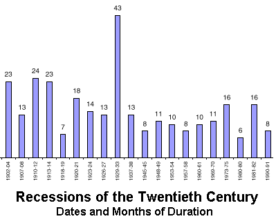
In the twentieth century there were 20 recessions in
the United States.

The last recession of the 20th century ended in 1991
and the US, are enjoyed it longest recovery ever. . .
until March 2001 when we experienced a short recession.
In 2008 the US economy entered another reseccion where
unemployment reached around 10%
OPTIONAL: Table listing dates and length of business
cycle recessions and recoveries - http://www.nber.org/cycles.html
Outline of Chapter 6: Macroeconomic Concepts and the
role of Price "Stickiness"
1. How well is the economy doing?
a. Real GDP (real Gross Domestic Output)
(1) nominal GDP
(2) real GDP
b. Unemployment
(1) 5 Es Definition
(2) Common Definition
c. Inflation
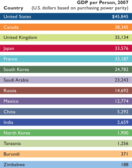
2. The Miracle of Modern Economic Growth
a. growth before the industrial revolution
(1) output growth
(2) output per capita growth
(3) result:
(a) no change in living standards
(b) little difference between living
standards
b. modern economic growth
(1) industrial revolution: output grows
faster then population
(a) not all countries
(b) even small increases in output result in
large increases oin living standards over
time
- rule of 70

- If a $10,000 GDP per capita increases by
2% a year
- how long will it take to double to
$20,000
- how long will it take to quadruple to
$40,000
- how long will it take to reach
$80,000
(c) results in vast differences inliving
standards

3. Savings, Investment, and Choosing between Present
and Future Consumption
a. Review: Production Possibilities Model:
Present Choices Future Possibilities
b. Savings
c. Investment
(1) financial investment
(2) economic investment
d. economic investment is ultimately limited by the
amount of savings, and more savings now depends on
less consumption now
e. the role of banks
4. Uncertainty, Expectations, Demand Shocks, and
Supply Shocks
a. definitions
b. demand shocks and flexible prices: producing the
full employment output
c. demand shocks and sticky prices: fluctuations in
GDP and employment
5. How Sticky are Prices?
6. Macroeconomic models and Price Stickiness
A Model of the Macro Economy: Aggregate Demand (AD)
and Aggregate Supply (AS)
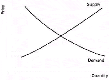
We have already discussed the Supply and Demand
model to determine individual prices and quantities. That
was a microeconomic model. The key word is "individual"
product or "individual" industry.
In macroeconomics we study the whole, or "aggregate",
economy. Our new AGGREGATE supply and AGGREGATE demand
model looks similar to the supply and demand model, but
they are NOT the same! We are now discussing the whole
economy, so AD is the demand for all products in an
economy and AS is the supply of all products.
|
Supply and Demand for an INDIVIDUAL
product
|
AGGREGATE Supply and AGGREGATE
Demand
|
|

|

|
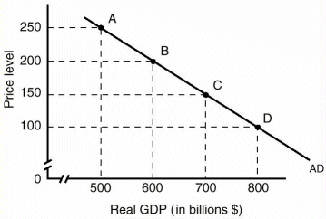
Aggregate Demand
Definition
Aggregate demand is the demand of all products in an
economy - OR the relationship between the Price Level and
the level of aggregate output (real GDP) demanded.
Be able to define:
- Aggregate Demand
- Real Domestic Output (RDO) which can be measured
by real GDP
- real GDP
- Price Level

Graphically: down-sloping -- why?
Economists have three explanations of why the AD
curve is downward sloping from left to right. They are:
- the real-balances (wealth) effect
- the interest-rate effect
- the foreign purchases effect
We want to understand why if the Price Level increases
the amount of aggregate output (real GDP) demanded
decreases. Why is the AD curve downward sloping from left to
right?
Price Level 
 Amount
of output demanded Amount
of output demanded 
We always want to understand why the graphs that we use
in economics have the shapes that they do? Are their shapes
realistic?
The real-balances (wealth) effect:
When the average level of prices in the economy
increases, why do consumers, governments, business and
foreigners purchase less?
One reason is the wealth effect. When the price level
in the economy increases what happens to the real value,
or the purchasing power, of financial assets (of money
you have saved) and why do we then buy less?
Price Level 
 real value of financial
wealth ?
  Amount of output demanded
Well, when the
Price Level 
 real value of financial
wealth
 Amount of output demanded
because they now have less real wealth.
The interest-rate effect:
When the average level of prices in the economy
increases, why do consumers, governments, business and
foreigners purchase less?
Another reason is the interest rate effect. When the
price level in the economy increases what happens to the
interest rates and why do we then buy less ?
Price Level 
 interest rates ?
 Amount of output demanded
Well, when the
Price Level 
 interest rates

 Amount of output demanded
because people will buy less of those things for
which they have to borrow money.
The foreign purchases effect :
When the average level of prices in the economy
increases, why do consumers, governments, business and
foreigners purchase less?
The third reason is the foreign purchases effect. When
the price level in the US economy increases what happens
to the relative prices of foreign products and why are
fewer American products purchased ?
Price Level 
 relative price of foreign
products ?
  Amount of output demanded
Well, when the
US Price Level 
 relative price of foreign
products
 Amount of US output demanded
because people will now buy more of the now
relatively cheaper foreign products.
Changes in AD
Just like with supply and demand in the individual
product market, there are determinants that will shift the
AS and AD curves. These determinants are the REAL WORLD
EVENTS that cause the graphs to shift. remember, that our
goal is to better understand what causes the business cycles
-- or what causes UE, IN, and EG to change.
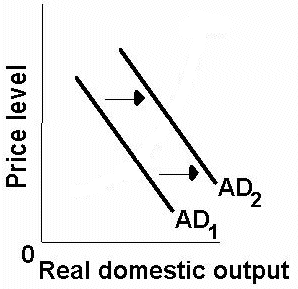
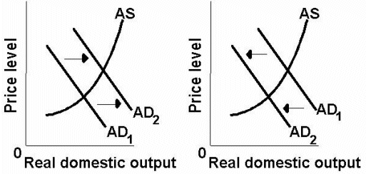
Increase in AD
(shifts to the right)
|
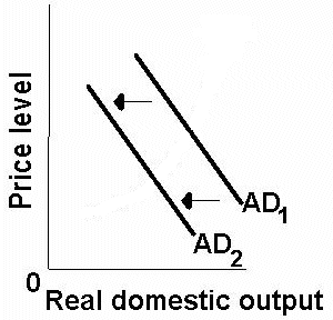
Decrease in AD
(shifts to the left)
|
|

|

|
In the following discussion the double arrow ( )
means "causes". It is important that you get the
cause-effect in the correct order. The direction of the
arrow matters )
means "causes". It is important that you get the
cause-effect in the correct order. The direction of the
arrow matters
Just like with demand in the individual product market,
there are determinants of AD that, if they change, will
shift the AD curve. They are:
- change in consumer spending (C)
C 
  AD
AD
C 
  AD
AD
- change in Investment spending (I)
(Note: "Investment" does NOT mean buying stocks and
bonds. Investment occurs when business buy capital.
Remember that capital is NOT money. Capital is a
manufactured resources. capital is something that is
produced that is used to produce something else. So if I
buy 100 shares of Stock in Microsoft, that is NOT and
investment, but if a carpenter buys a hammer, or if
Microsoft builds a new office building, THAT is an
"investment".)
I 
  AD
AD
I 
  AD
AD
- change in Government purchases (G)
G 
  AD
AD
G 
  AD
AD
- change in Net Exports (Xn)
Xn 
  AD
AD
Xn 
  AD
AD
- change in Money Supply (S)
MS 

 Interest Rates
  I
I 
  AD
AD
MS 

 Interest Rates
  I
I 
  AD
AD
- change in Taxes (T)
T 

 C
C 
 AD
AD
T 

 C
C 
 AD
AD
- change in Saving (S)
S 

 C
C 
 AD
AD
S 

 C
C 
 AD
AD
Summary of the determinants of AD:
But what causes these things to change? Well, economists
have identified some determinants of the main components of
spending: C, I, G, and Xn.
Determinants of C, I, G, and Xn:
C = consumer spending (and saving)
1. consumer wealth
Wealth  
 C
C 
 AD
AD
Wealth  
 C
C 
 AD
AD
2. consumer expectations
Expected future Income 

 C today
 AD today
Expected future Income 

 C today
 AD today
3. consumer indebtedness
Consumer Debt 

 C
C 
 AD
AD
Consumer Debt 

 C
C 
 AD
AD
4. taxes
T 

 C
C 
 AD
AD
T 

 C
C 
 AD
AD
I = investment spending
1. interest rates (money supply)
MS 

 Interest Rates
  I
I 
  AD (memorize this, it will help in
future chapters)
MS 

 Interest Rates
  I
I 
  AD
AD
|
I know the textbook does not mention
"money supply", but it will in unit 3. So,
we might as well learn it now.
|
2. profit expectations on investment projects
profit expectations 
 I
I 
  AD
AD
profit expectations 
 I
I 
  AD
AD
3. business taxes
Business Taxes 

 I
I 
 AD
AD
Business Taxes 

 I
I 
 AD
AD
4. technology
technology 
 I
I 

 AD
AD
5. degree of excess capacity
excess (unused) plant capacity 

 I
I 
 AD
AD
excess (unused) plant capacity 

 I
I 
 AD
AD
G = government purchases
Xn = net export spending
- net income abroad
Income in Foreign Countries 

 Xn
Xn 
 AD
AD
Income in Foreign Countries 

 Xn
Xn 
 AD
AD
- exchange rates
value of the US dollar 

 Xn
Xn 
 AD
AD
value of the US dollar 

 Xn
Xn 
 AD
AD
Aggregate Supply (AS)
Definition
Aggregate Supply is the supply of all products in an
economy - OR the relationship between the Price Level and
the level of aggregate output (real GDP) supplied.
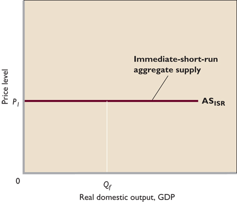
Immediate Short-Run AS
Assumption: both input prices and output
prices are fixed (do not have time to chnge)
How long it is depends on the type of firm
Input price can be fixed in the immediate short run
and in the short run by contracts. for example labore
unions sign two year contracts and their wages won't
change until the end of the contract.
Output prices are fixed only in the immediate short
run. Usually this is because firms set their prices
for their customers and then agree not to change them
for awhile.
Result:
How much is supplied then depends only on
how much is spent (aggregate spending) and the AS
curve is horizontal.

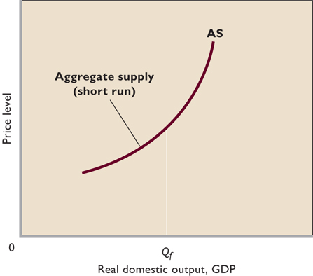
Short Run AS
Assumtion: input prices are fixed, or highly
inflexible, as explained above, but output prices can
change.
Note that not all input prices are completely
fixed, some can change a bit.
Graph is upward sloping because if the price level
increases (i.e. people are willing to pay more for
products), this will increase profits of firms
(because revenues are higher, but imput prices are
fixed). So at the higher price level and therefore
higher profits, businesses will produce more.
Why is the graph "curved" upwards will be explained
below.

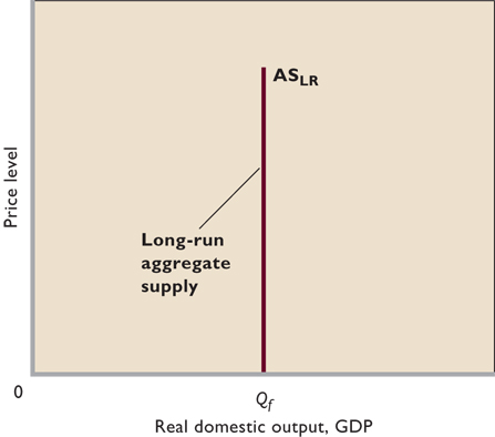
Long Run AS
Assumption: both input and output prices are
flexible.
AS graph is vertical meaning that in the long run
the economy will produce the full employment level of
output no matter what the price level is. Why?
If people are willing to buy more by
paying more you would think that firms will want to
produce more. But if in order to produce more they
must also pay more for resources (since all are
already being used and they will have to pay more
to draw them away from other firms) then input
prices will rise and there is no increase in
profits to encourage firms to produce more.

A combined (simplified model)
The textbook says
"The immediate-short-run aggregate supply curve,
theshort-run aggregate supply curve, and the long-run
agregate supply curve are all important. . . . But our
focus in the rest of this chapter and the several
chapters that immediately follow will beon the short-run
aggregate supply curve. . . . our emphasis on the
short-run agregate supply curve stems fromour interest in
understanding the business cycle in the simplest possible
way. It is a fact that real-world economices typically
manifest simultaneous changes in both their price levels
and their levels of real output."
Graphically
Graphically, we would expect the AS curve to be
upward sloping. If businesses can get a higher price for
their products (higher price level) then they will want
to produce MORE. So the AS curve should be upward
sloping.
But, remember that the price level is the
average level of ALL prices in the economy, therefore, if
the price level increases, the price of resources will
also increase. Higher resource prices will encourage
businesses to produce LESS. So maybe the AS curve should
be downward sloping????
Some economists graph the AS curve like in the graph
below to handle this problem:

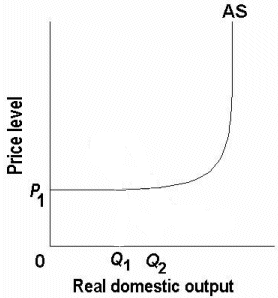
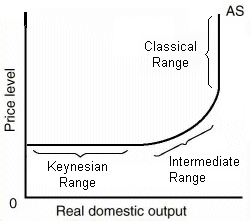
Shape
We can identify three different parts, or
ranges, to the AS curve:
1. Keynesian (horizontal) range
2. classical (vertical) range
3. intermediate (up-sloping) range

In the Keynesian or horizontal range the level of
output in the economy is low. Very little is being
produced so there are a lot of resources NOT being used.
Businesses are therefore able to produce more output
without having to pay more for the additional resources.
Since many resources are unemployed, businesses will not
have to pay a higher price to employ them. Therefore,
they can produce more without having to raise the price
(note how the price level is constant (does not increase)
in the Keynesian range of the AS curve.
In the Classical or vertical range of the AS curve
there are no more resources available. ALL are being
used. So all businesses together cannot produce any more
since there are no more resources to use. But, if some
businesses try to produce more by enticing resources away
from other businesses with higher resource prices (higher
wages for example) they will have to raise their prices
to cover the higher costs - BUT the amount produced in
the whole economy will stay the same since no additional
resources are being available. So, the AS curve is
vertical indicating no additional output even at higher
price levels.
In the intermediate range the AS curve begins to rise
slowly as a few resources begin to run out and at higher
levels of output the AS curve becomes steeper as the
economy runs out of even more resources, until it is
vertical when all resources are being used and it is not
possible to produce any more output.
Aggregate Supply and Full Employment
If we want to use the AS-AD model to better
understand the macroeconomic issues of UE, IN. and EG,
then we need to be able to locate the "full employment
level of output" - the amount of GDP that can be produced
if all resources are being used.
You would think that this would occur where the AS
curve is vertical, but what do we really mean by "full
employment"? Does this mean all resources, including
labor, working everyday day for as many hour as is
physically possible? Or does it mean "full employment"
under "normal" conditions where people work maybe 40
hours a week? They retire at age 65 and don't begin to
work until age 18 or 22? If this is our definition of
"full employment", then it would be possible to produce
more than the full employment level of output by having
people work 50, 60, 70, 80, or even more hours a week.
People could never retire and just keep working until
they die, etc. If this happened then MORE would be
produced. But this isn't really what we mean when we say
"full employment". Therefore, it is possible to produce
more than the "normal" full employment level of
output.
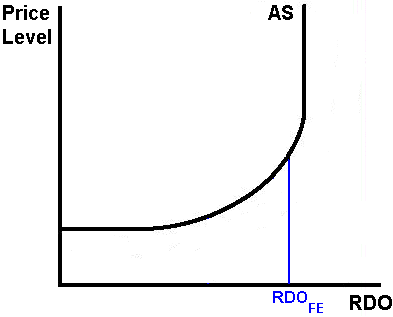
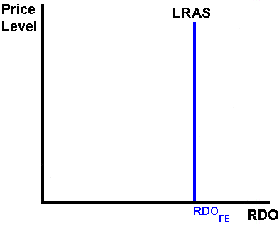
The graph below shows how we can illustrate this level
of output under normal conditions of full employment.

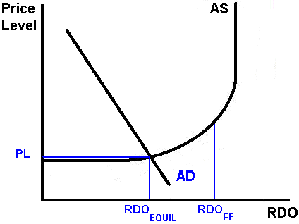
Note that at levels of output beyond the full
employment level (beyond RDO-FE) the price level
increases dramatically resulting in high inflation,
therefore some people define the full employment level of
output as the amount of output that can be produced and
still maintain low inflation.
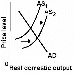
Changes in AS
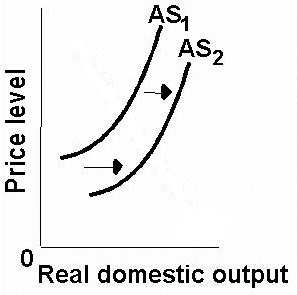
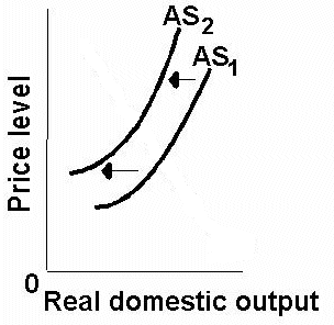
Increase and decrease in AS
Increase in AS
(shifts to the right)
|
Decrease in AS
(shifts to the left)
|
|

|

|
Determinants of AS
Just like with supply in the individual product
market, there are determinants of AS that, if they
change, will shift the AS curve. They are:
a. change in input prices
price of resources 

 AS
AS
price of resources 

 AS
AS
1) labor
2) land (OPEC)
[OPTIONAL: http://news.bbc.co.uk/hi/english/business/the_economy/newsid_300000/300492.stm]
3) capital
4) entrepreneurial ability
b. changes in the productivity of resource
productivity 

 AS
AS
productivity 

 AS
AS
Be sure to know the difference between:
1) Productivity
- output per unit of resource
2) production
- the quantity produced
3) productive efficiency
- producing at a minimum cost (5 Es)
c. legal-institutional environment
business taxes and gov't red tape


 AS
AS
business taxes and gov't red tape 

 AS
AS
1) business taxes and subsidies
2) government regulation (red-tape)
Summary of the Determinants of AS
Macroeconomic Equilibrium
Equilibrium
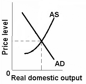
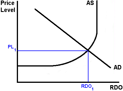
You can use the AS-AD graph to find the
equilibrium price level and the equilibrium level of
output. We can then figure out what happens to US, IN and
EG. The equilibrium level of output ant he equilibrium
price level will occur where the two lines cross.

In this economy the level of real domestic output
(real GDP) will move toward RDO1 and the price level will
move toward PL1.
Changes in AD and the Macroeconomic Issues
The reason we have developed the AS-AD model is to better
understand UE, IN, and EG.
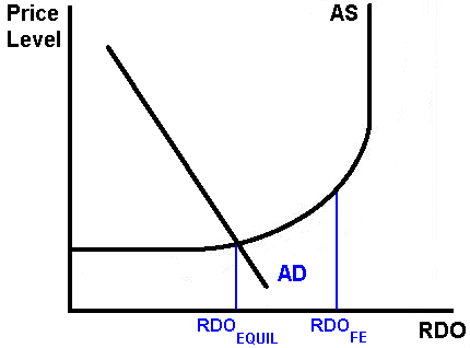
Employment

If the equilibrium level of output is below the full
employment level as in the graph above the result is
unemployment.
Inflation
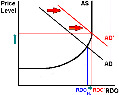
Demand-pull inflation is inflation caused by an
increase in AD. As you can see on the graph below, if
there is an increase in AD the price level increases.
Inflation is the rate of increase in the price level.

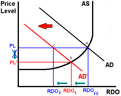
A decrease in AD will cause the level of output to
decline indicating higher unemployment.
But what happens to the price level when AD decreases?
Normally we would expect the price level to decline from
PL to PL' on the graph below if AD decreases, but can you
remember a time when the price level (the average level
of ALL prices in the economy) decreased? It doesn't
happen very often. Business are more willing to raise
their prices (causing more inflation) than they are to
decreases their prices (causing deflation). Economists
call this the ratchet effect. Like a ratchet that
only works in one direction, prices more easily move in
one up than down. Sometimes it is said that prices are
"sticky downwards".
On the graph then, if AD decreases instead of going
from "a" to "b" (less output and a lower price level),
the economy goes from "a" to "c" since prices are sticky
downwards and tend not to decrease. Therefore the price
level stays the same (at PL), but the level of output
drops even more (from RDO-FE to RDO2 instead of only to
RDO1).

The causes of the ratchet effect are listed below. For
several reasons businesses are reluctant to lower prices
even when faced with lower aggregate demand.
a) Wage contracts often mean that
businesses have to increase their costs even if AD
decreases.
b) If businesses lower wages so that they can lower
their prices, this may have an adverse effect on
morale and productivity
c) If businesses lower wages so that they can lower
their prices, they may lose some of best workers in
which they have invested much in
training
d) To lower their prices business would like to
decrease their labor costs (wages), but they may not
be able to because of the minimum wage
laws.
e) Some firms may fear price wars meaning if
they lower their price, then their competitors will
match their price decrease or even lower their prices
even more.
f) Finally, businesses may have monopoly
power, giving them more control over their prices
and they may choose to take smaller profits rather
than lowering their prices.
Changes in AS and the Macroeconomic Issues
A decrease in AS would decrease output and raise the
price level. This would result in more unemployment and more
inflation. We call this inflation "cost-push" inflation. It
is inflation caused by a decrease in AS.

Stagflation
A decrease in AS results in "stagflation". Stagflation
is a decrease in output (an increase in unemployment)
accompanied by an increase in inflation - a STAGnant
economy with inFLATION. It is caused by a decrease in
AS.
An increase in AS would increase output and lower the
price level. This would result in less unemployment and
less inflation.

Economic Growth
What about economic growth? Our textbook
discusses three definitions of economic growth
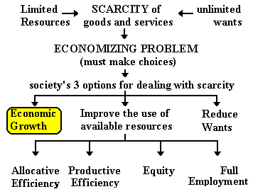
- Increasing our POTENTIAL OUTPUT (chapter 1; the
5Es definition)
- Increasing Output, (chapter 8)
- Increasing Real GDP per capita (chapter
8)
(1) Increasing our POTENTIAL OUTPUT
I like to call this increasing our ABILITY to
produce. This is the definition we used in the
5 Es
lesson. This is the most fundamental definition of
economic growth. It is the type of economic growth
used on our 5 Es diagram.

We can increase our ABILITY to produce goods and
services (or increase our POTENTIAL GDP) if we
get:
- more resources
- better resources, and
- better technology
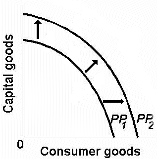
Since this increases maximum output that we are
able to produce it shifts the PPF outward. On the
graph below, economic growth would cause the PPF to
move from PP1 to PP2.

This doesn't necessarily mean that the economy IS
producing more, just that it CAN produce more. To
achieve our new potential levels of output we also
need full employment and productive efficiency. It
could be possible to have this type of economic growth
so that we CAN produce the quantities represented by
point E, but if there is unemployment and productive
inefficiency we would be at a point beneath this new
curve (maybe point C). So we may get new resources or
new technology so we CAN produce more (point E on
PP2), but if we don't use the new resources (i.e. we
have unemployment) or if we don't use the new
technology (i.e. we have productive inefficiency) , we
may remain on PP1 (point C).
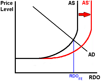
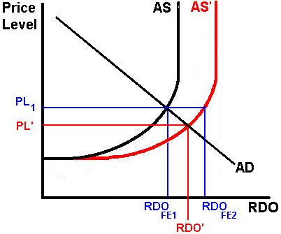
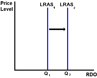
In the AS-AD model INCREASING OUR POTENTIAL OUTPUT
is represented by in INCREASE IN AS.

Notice that when AS increases, the full employment
level of output increase from RDO-FE1 to RDO-FE2. This
is an increase in our potential level of output.
In the 5 Es lecture we said that economic growth is
caused by:
- more resources
- better resources, or
- better technology
An increase in the production possibilities curve
is caused by having more resources, better resources,
or better technology.
An increase in AS is caused by:
- a decrease in the price of resources
- an increase in productivity
- lower business taxes and government red
tape
These are all really the same thing.
(2) Increasing Output (increasing real GDP)
The most commonly used definition of economic
growth is simply producing more. (Later we will call
this INCREASING REAL GDP.) When an economy increases its
output it is often said to have achieved economic growth.
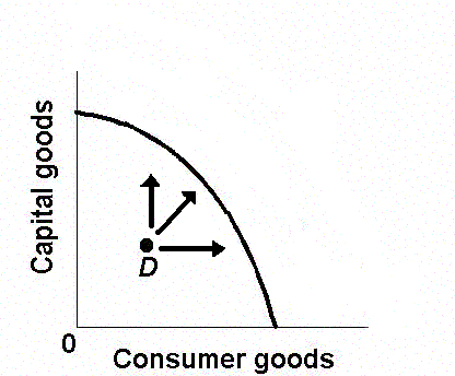
But if by producing more we are simply ACHIEVING OUR
POTENTIAL, then we could also say that it is REDUCING
UNEMPLOYMENT or ACHIEVING PRODUCTIVE EFFICIENCY. On our
production possibilities graph this would be represented
by moving from point D to a point on the curve.

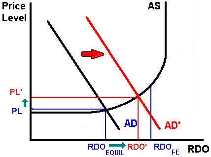
On our AD-AS model we could illustrate this type of
growth (achieving our potential) by an increase in
AD.

Notice that output increase from RDO-EQUIL to RDO',
but the full employment level of output, which is our
potential level of output, does not change (RDO-FE).

If AD increases so that the new equilibrium is at the
full employment level of output, it is analogous to going
from a point inside the production possibilities curve to
a point on the curve.
(3) Increasing Real GDP per capita
This means increasing output per person. GDP per
capita is calculated by dividing output by the
population.
SUMMARY OF THE TYPES OF ECONOMIC GROWTH
|
ECONOMIC GROWTH
Increasing output by INCREASING THE
POTENTIAL
(Called "economic growth" on our 5Es model)
|
ECONOMIC GROWTH
Increasing output by ACHIEVING THE
POTENTIAL
(Called "reducing unemployment" on our 5Es
model)
|
|


|


|
Using the AS / AD Model
Now that we have introduced the AS / AD model, let's
learn how to use it. The exam 2 extra credit essay
question will be a lot like these examples.
EXAMPLE 1
Read this short article from cnnfn.com.
Analyze the article by:
(1) Identifying the determinants of AD and/or AS
that have changed.
This is important. It all begins with a CHANGE in one of
the determinants of AD or AS. You MUST memorize these
determinants and know which ones shift the AD curve and
which shift the AS curve!
(2) Then graph the changes on the AS-AD model.
Next, you must know which way the determinants will shift
the curve.
(3) Finally use your graph to discuss has happened to
UE, IN, and EG.
|
|
German
GDP grows 0.7%
|
|
Export
increase lifts economy; OECD raises
estimate of growth rate
|
|
May
30, 2000: 7:08 a.m. ET
|
|
|
LONDON (CNNfn) - German first-quarter
gross domestic product increased 0.7
percent from the previous three-month
period, as expected, helped by demand
for exports, the Federal Statistics
Office said on Tuesday.
The German economy, Europe's biggest,
expanded by 3.3 percent in the first
quarter of 2000 compared to the same
period a year ago, the strongest annual
rate of growth since the first quarter
of 1998.
The quarter-over-quarter growth rate
matched the 0.7 percent pace recorded
in the three months ended Dec. 31,
aided by a decline in the euro that has
made exports cheaper. Economists now
predict full-year growth of more than 3
percent.
"It's a very good start to the year
2000 and clearly indicates the upswing
is intact and growth is accelerating,"
said Manuela Preuschl, an economist at
Deutsche Bank in Frankfurt.
The Organization for Economic
Cooperation and Development Tuesday
raised its forecast for German economic
growth, predicting GDP would rise 2.9
percent this year and 3 percent in
2001, as exports remain strong and tax
cuts boost domestic demand.
In the first quarter, exports grew 15.3
percent from a year earlier while
imports rose 11.9 percent. Gross
investment in plant and equipment
increased 5.7 percent. The pace of
growth in private consumption weakened
to 0.9 from a year earlier, compared
with 2.2 percent in the fourth quarter
of 1999.
--from staff and wire reports
|
|
Original AS/AD graph:

Determinants that are mentioned in the article:
"German
first-quarter gross domestic product increased 0.7
percent from the previous three-month period, as
expected, helped by demand for exports, the
Federal Statistics Office said on Tuesday."
So: Xn 

 AD AD
ALSO:
"The
Organization for Economic Cooperation and Development
Tuesday raised its forecast for German economic
growth, predicting GDP would rise 2.9 percent this
year and 3 percent in 2001, as exports remain strong
and tax cuts boost domestic demand."
So:
 Taxes Taxes
 C
C    AD AD
Draw the changes on the graph:  AD
AD

What happened to UE, IN, and EG as a result of these
changes?
Since equilibrium RDO increased from RDOequil
to RDO' we can conclude that unemployment (UE)
decreased and economic growth (EG) increased. The
price level rose slightly from PL to PL' so maybe
inflation (IN) increased a little.
EXAMPLE 2
Read this short article from http://news.bbc.co.uk.
Analyze the article by identifying the determinants of AD
and/or AS that have changed. Then graph the changes
on the AS-AD model. Finally use your graph to discuss has
happened to UE, IN, and EG.
[http://news.bbc.co.uk/hi/english/business/the_economy/newsid_300000/300492.stm]
Again, be sure to follow the same three steps:
(1) Identifying the determinants of AD and/or AS
that have changed.
This is important. It all begins with a CHANGE in one of
the determinants of AD or AS. You MUST memorize these
determinants and know which ones shift the AD curve and
which shift the AS curve!
(2) Then graph the changes on the AS-AD model.
Next, you must know which way the determinants will shift
the curve.
(3) Finally use your graph to discuss has happened to
UE, IN, and EG.
|
Wednesday,
March 24, 1999 Published at 10:34 GMT


Business:
The Economy

OPEC
slashes oil production
Oil
producers finally agree to restrict
output

Ministers
from oil producing countries have agreed to cut
global production by 7% to bolster depressed oil
prices.
The
members of the Organisation of Petroleum
Exporting Countries (OPEC) and others meeting in
Vienna have agreed to a reduction in output of
2.1m barrels a day until April next
year.
Saudi
Oil Minister Ali al-Naimi said the new
restrictions were aimed at lifting oil prices
back to $18 a barrel within a year.
. . .
. . .
Inflation
fears
However,
this would hit consumers hard, perhaps
rekindling inflation.
The oil price has increased 30% in the last
month on the belief that OPEC would finally
agree to cap output. Oil has risen from its low
in December of below $10 a barrel, for Brent
crude for May delivery, to $13.75 as the
decision was announced.
. . .
. . . .
|
Original AS/AD graph:
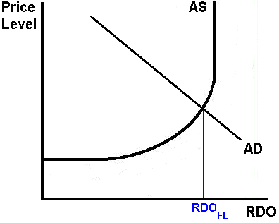
Currently the economy of the United States is
operating at the full employment level of output as shown
in the graph below:

Determinants that are mentioned in the article:
"The
oil price has increased 30% in the last month on the
belief that OPEC would finally agree to cap output.
Oil has risen from its low in December of below $10 a
barrel, for Brent crude for May delivery, to $13.75 as
the decision was announced."
So the determinant that has changed is the Price of
Resources:
Price of resources 

 AS
AS
Draw the changes on the graph:  AS
AS

What happened to UE, IN, and EG as a result of these
changes?
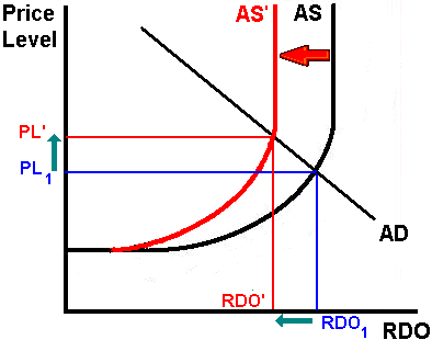
Since equilibrium RDO decreased from RDO1 to
RDO' we can conclude that UE increased and EG decreased.
The price level will rise from PL1 to PL' indicating
inflation. With output down and prices up, this increase
in oil prices may result in stagflation.
EXAMPLE 3
Is an increase in exports good for an economy? Most
students will quickly answer "yes" to this question, as
would most newspaper writers. But WE know better. It
depends.
Currently the economy of the United States is operating
at the full employment level of output as shown in the graph
below:

An increase in exports will do what to the graph above?
An increase in exports will increase AD.
GRAPH IT!

The result: INFLATION! So is an increase in exports good
for THIS economy? NO.
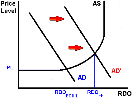
But, if initially the economy is experiencing high
unemployment like in the graph below:

Then, an increase in exports would increase AD and move
the economy closer to the full employment level of output
with only a little inflation. See graph:

This would of course be good for the economy. So is an
increase in exports good for an economy? - - It depends.
EXAMPLE 4
Now you try it. Read this short article from cnn.com.
Analyze the article by identifying the determinants of AD
and/or AS that have changed. Then graph the changes
on the AS-AD model. Finally use your graph to discuss has
happened to UE, IN, and EG.
Remember to:
(1) Identify the determinants of AD and/or AS
that have changed.
This is important. It all begins with a CHANGE in one
of the determinants of AD or AS. You MUST memorize
these determinants and know which ones shift the AD
curve and which shift the AS curve!
(2) Then graph the changes on the AS-AD model.
Next, you must know which way the determinants will
shift the curve.
(3) Finally use your graph to discuss has happened
to UE, IN, and EG.
MORE EXAMPLES / REVIEW:
For more exercises see: http://www.harper.cc.il.us/mhealy/eco212i/lectures/asad/adasprac.htm
Macroeconomic Policies
Now that we have this handy tool, let's use it to discuss
government policies (NOTE: when I use the term "policies", I
always mean "government policies"). What is the role of the
government in a market economy? In a market economy
(capitalist economy) the government has a limited role, but
some people believe that the government should try to help
the economy maintain full employment and low inflation. We
have discussed in the 5 Es lesson that unemployment results
in greater scarcity since some resources are not being used
so less will be produced. Government policies may be able to
help the economy achieve full employment and therefore
reduce scarcity.
In a previous chapter we discussed the five economic
functions of governments in capitalist economies. Here we
will begin our discussion of how to "promote stability".
|
Economic Functions of Government in a
Market (Capitalist) Economy
- Providing the legal structure
- Maintaining competition
- Redistributing income
- Reallocating resources
- negative externalities
- positive externalities
- public goods and services
- Promoting
stability
|
Stabilization Policies
Definition: government policies design to reduce
unemployment (UE) and/or inflation (IN). All the policies
discussed here can be classified as stabilization
policies.
There are two major types of stabilization
policies:
- demand-management policies
- supply-side policies
Demand-Management Policies
Definition: Policies design to shift the AD
curve in order to reduce unemployment or to reduce
inflation.
Tools -- Some of the determinants of AD can be
manipulated by the government to achieve these goals.

There are two types of demand-management policies
depending upon WHO conducts the policy:
- fiscal policy is undertaken by the
president and the congress, and
- monetary policy is undertaken by the
Federal Reserve Board (often called the "fed").
FISCAL POLICY
There are two types of fiscal policy:
- expansionary fiscal policy
- contractionary fiscal policy
The goal of expansionary fiscal policy is to reduce
unemployment. Therefore the tools would be an increase in
government spending and/or a decrease in taxes. This
would shift the AD curve to the right increasing real GDP
and decreasing unemployment, but it may also cause some
inflation.
The goal of contractionary fiscal policy is to reduce
inflation. Therefore the tools would be an decrease in
government spending and/or an increase in taxes. This
would shift the AD curve to the left decreasing
inflation, but it may also cause some unemployment.
MONETARY POLICY
There are two types of monetary policy
- easy money
- tight money
The goal of an easy policy is to reduce unemployment.
Therefore the tool would be an increase in the money
supply. This would shift the AD curve to the right
decreasing unemployment, but it may also cause some
inflation.
MS 
 ¯ Interest Rates
  I
I 
  AD
AD
The goal of a tight money policy is to reduce
inflation. Therefore the tool would be a decrease in the
money supply. This would shift the AD curve to the left
decreasing inflation, but it may also cause some
unemployment.
MS 

 Interest Rates
  I ¯
I ¯
 ¯
AD ¯
AD
"Supply-Side Economics"
Supply-Side economic policy occurs when the government
tries to increase the AS curve. this will reduce both
unemployment and inflation.

There are three determinants of AS:
a. change in input prices
price of resources 

 AS
AS
b. changes in the productivity of resource
productivity 

 AS
AS
c. legal-institutional environment
business taxes and gov't red tape 

 AS
AS
Supply-Side Policies
Supply-side policies try to increase
productivity. Often this includes less government
regulations. Also, in the 1980s President Reagan
decreased marginal income tax rates as a supply-side
policy (sometimes called "Reaganonmics"). The idea was
that people will work more if they can keep more of
their income
We have said that decreasing income taxes will
INCREASE AD. But here we said that it may also
INCREASE AS. Which is it? both may be true, but the
effect on AD is probably quicker. In this class a tax
cut will increase AD, UNLESS we mention that is is a
"supply-side" tax cut. Then we will increase the AS
curve.
REVIEW
More on the Long-Run Aggregate Supply
Definition: Short-run and long-run.
For macroeconomics the short-run is a period in which
wages (and other input prices) do not respond to price
level changes because workers may not be fully aware of
the change in their real wages due to inflation (or
deflation) and thus have not adjusted their labor supply
decisions and wage demands accordingly or employees hired
under fixed wage contracts must wait to renegotiate
regardless of changes in the price level.
In the long run the aggregate supply curve is vertical
at the economy's full-employment output. The curve is
vertical because in the long run resources prices adjust
to changes in the price level, leaving no incentive for
firms to change their output.


Why is the long run aggregate supply curve vertical?
Let's see what happens first in the short run
(assuming wages do not change), and then see what happens
when wages do change. (Note: when wages change the short
run aggregate supply curve will change - this is the
price of resources determinant.)
INFLATION
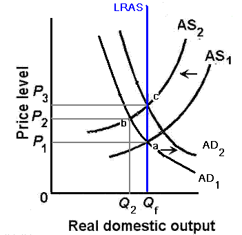
Let's begin by seeing what happens if there is
demand-pull inflation. If AD increases it will in the
short run increase the price level and increase real
output. On the graph below this can be illustrated as an
increase of AD from AD1 to AD2 and the equilibrium point
moves from "a" to "b". So the price level rises from P1
to P2 and output increases from Qf to Q2. (Note that Qf
is the "full employment level of output.) Earlier we
discussed how an economy can produce more than the full
employment level of output.
What happens when workers see that prices are rising
but their wages are staying the same? Remember, by
definition, in the short run wages do not change, but
they can in the long run. An economy can temporarily
produce more than the full employment level as people
work more than they want to, but in the long run they
will demand higher wages. When wages increase this will
be an increase in the price of resources and the the
short run AS curve will decrease, shift to the left. On
the graph below this is a movement from AS1 to AS2 and
the economy moves from point "b" to point "c". This
causes the price level to rise from P2 to P3 and the
level of output decrease back to the full employment
level (from Q2 to Qf). The long run result is that the
level of output in the economy has stayed at Qf and the
price level has risen. The long run aggregate supply
curve is therefore vertical (the blue line below).

What happens in the long run if in the short run there
is cost-push inflation? Cost push inflation is caused by
increases in the cost of production at each price level
maybe caused by the increase in the price of a key
resource. This shifts the short run supply to the left on
the graph below from AS1 to AS2. the result is that the
economy moves from point "a" to point "b" and there is a
recession (unemployment increases) and inflation. Earlier
we called this "stagflation". What should the government
do?
If government attempts to maintain full
employment by using expansionary fiscal or monetary
policy to increase AD (from AD1 to AD2 on the graph
above) an "inflationary spiral" may occur. If
government doesn't do anything when there is cost push
inflation, a recession will occur with high
unemployment and a loss of real output.
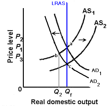
RECESSION
When aggregate demand shifts leftward a recession
occurs. Let's see what will happen in the short run
and in the long run. If prices and wages are
downwardly flexible, the price level will fall form P1
to P2 when AD decreases from AD1 to AD2. With the
price level falling the real wages of workers (i.e.
the purchasing power of their wages) increases. It's
as if they are being paid more. Since businesses are
selling less and getting less, but workers are getting
more, business owners will want to reduce the wages of
their workers restoring their purchasing power to what
it was before the recession started. This decrease in
wages will cause an increase in the short run AS
(price of resources determinant) and the economy will
move from point "b" to point "c". So, in the long run
(remember that "long run" means that wages have time
to change) the economy is back at the full employment
level of output but the price level is lower. Again,
the long run aggregate supply curve is vertical.
This is the most controversial application of this
new "extended" AD-AS model. The key point of dispute
is how long it would take in the real world for the
necessary price and wage adjustments to take place to
increase AS and bring the economy back to full
employment. If policy makers think that it will take a
long time to move back to full employment then they
may want to enact some expansionary fiscal or monetary
policy. BUT, if the prices and wages change quickly,
then the government does not have to do anything. If
there is a recession they can just wait a short time
and the economy will quickly adjust back to full
employment.
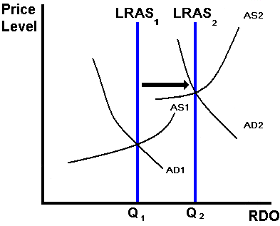
Economic Growth and the Long Run Aggregate Supply
Now we can add another graph to illustrate
economic growth
|
