 |
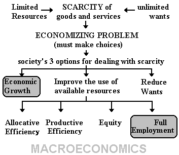
In unit 3 we will discuss macroeconomic POLICY. The term "policy" implies that the government is attempting to influence the macroeconomy. The issues discussed in macroeconomics are:
1. full employment
2. price stability
3. economic growth
In the week 1 online lecture "The 5 Es of Economics" we discussed the importance of these topics in reducing scarcity and receiving the maximum satisfaction possible from our limited resources.
|
|
Here we will look at what the government can do to reduce unemployment or reduce inflation. We will study fiscal policy in chapters 10 and 13 and monetary policy in chapters 14, 15, and 16.
In chapter 10 we will look at the following three basic macroeconomic relationships to better understand how fiscal policy works.
1. Income and consumption, and income and saving. (We will look at this first)2. The interest rate and investment. (We will look at this last.)
3. Changes in spending and changes in output. (This is the most important relationship that we study in this chapter.)
The following is from the Aggregate Supply / Aggregate Demand (chapter 12) lecture.
SO, WE ALREADY KNOW:
If there is UE?
- increase G
- decrease T
- or do both
If there is IN?
- decrease G
- increase T
- or do both
NOW, WE ARE GOING TO LEARN:

So we already know that if there is unemployment the appropriate fiscal policy would be to increase government spending and/or decrease taxes. Here we will discuss HOW MUCH should government spending be increased or taxes cut?
From chapter 7 we know the expenditures approach to calculating GDP:
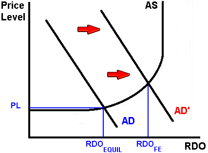
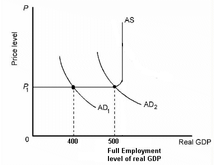
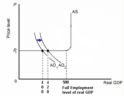
GDP = C + Ig + G + Xn 400 Look at the graph to the right and the formula above. You
can see that this economy is at equilibrium producing an
output of $400, but if there were full employment, a real
GDP of $500 could be achieved. Therefore, this economy has
an unemployment problem and is not producing as much as it
could. What is the appropriate fiscal policy could the
government use to move this economy to full
employment?
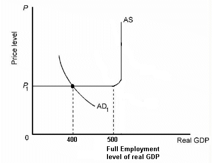
We know that the government could increase government spending and/or reduce taxes to increase AD and achieve full employment. Here, let's just concentrate on government spending.
By HOW MUCH should government spending be increased to achieve and equilibrium of $500 and full employment?
|
GDP |
= |
C |
+ |
I |
+ |
G |
+ |
Xn |
|
to $100 |
? |
One would think that if government spending was increased by $100 that GDP would go up by $100, BUT THIS IS NOT THE CASE! What we are going to learn in this chapter is that a small initial increase in spending results in a much larger change in GDP. This is called the MULTIPLIER EFFECT. A small initial change in spending will result in a larger change in GDP as the spending change works it way through the economy.
The Multiplier Effect: (How the multiplier process works)
This is because an initial change in spending will cause an initial increase in GDP and it also becomes income to someone else. (If I buy a new car, people who built and sold that car earn income equal to the price of the car.) What will these people do with their additional income? Well, they will spend some and save some. The amount that they spend increases GDP even more AND it also becomes income to someone else. These other people will spend some of this additional income and save some. The amount THEY spend increases GDP again and becomes income to someone else. This is called "induced consumptions" or consumption caused by an increase in income. This process continues so that the TOTAL change in GDP is much larger than the initial change in spending. See graph below.
This multiplier process helps explain why cities want the Superbowl, political conventions, or the Olympics to be held in their town. It's not just because these activities bring in people who will spend money and create jobs, but more importantly, this initial change in spending begins the multiplier process so that the total economic effect, and the number of jobs created ,is much larger than the initial spending on these activities alone would cause.
Read this article from the Philadelphia Inquirer newspaper (http://home.phillynews.com/gop/news/impa110698.asp). the Republican National Convention was held in Philadelphia in 2000 and in San Diego in 1996. It is clear that civic leaders understand the multiplier effect when they discuss "spinoff benefits".
------------- ------------------ --------------------- ------------------ --------------------- ---------
The Philadelphia Inquirer, November 6, 1998
Plentiful gains seen from GOP
The publicity for the city may be priceless. The visitors' spending could reach $300 million.
By Howard Goodman
INQUIRER STAFF WRITER
When the elephants thunder into Philadelphia in 2000, the vibrations are expected to shake an incredibly bountiful money tree, showering dollars all over the region.
The economic impact of the Republican National Convention will almost certainly exceed $125 million in direct spending on hotel rooms, meals and the like, along with at least $175 million in spinoff benefits (emphasis added), David L. Cohen said yesterday. Cohen, Mayor Rendell's former chief of staff, is cochairman of Philadelphia 2000, the committee formed to woo a political convention.
The estimate is based on a Federal Reserve Board study of the economic blessings felt in Chicago from the 1996 Democratic convention, with a little extra figured in for four years' worth of inflation, Cohen said.
"There is no convention you can host that has a greater economic impact than a national political convention," he said. "Most people agree the only thing you can host that has a greater economic impact is the Olympics."
. . . . .In San Diego, where the Republicans last met, business leaders still bask in the 1996 convention's glow. "We look at the convention as a week-long television commercial for your city as a destination," Salvatore Giametta, a spokesman for the San Diego Convention and Visitors Bureau, said in an interview this summer.
. . . . .
According to the Greater San Diego Area Chamber of Commerce, the four-day convention attracted 30,000 visitors who spent $26 million on hotel rooms. But there has been no follow-up study to show the convention's broader effect on the San Diego economy.
Despite the lack of data, San Diego "absolutely" would host a convention again, Giametta said. "We think it was good for the tourism industry without a doubt."
Brian Ford, an accountant for Philadelphia 2000, said that insisting on a study to prove that Philadelphia will benefit mightily from the GOP meeting "is like saying you need a study to show that a car works.". . . . .
Above we said that the multiplier works "because an initial change in spending will cause an initial increase in GDP and it also becomes income to someone else. (If I buy a new car, people who built and sold that car earn income equal to the price of the car.) What will these people do with their additional income? Well, they will spend some and save some. The amount that they spend increases GDP even more AND it also becomes income to someone else." This process then goes on and on . . . but why does it eventually stop or does it go on forever? If you reread the explanation of the multiplier process above you will get a clue as to why the process eventually stops. Notice that we said "What will these people do with their new income? Well, they will spend some and save some." People do not spend 100% of any additional income that they receive. the spend some and SAVE SOME. So that the additional spending is less than their increase in income. And when this additional spending becomes income to someone else, they sill save some and spend even a smaller amount. This will continue until the total change in savings is equal to the initial increase in spending. When this occurs there is nothing left to spend and the process stops.
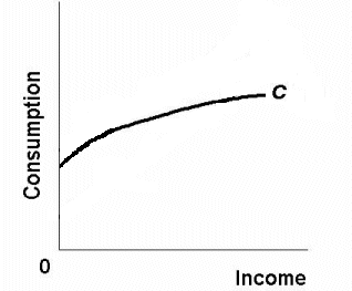
To understand the multiplier process we must gain a better understanding of how consumption and saving respond to changes in income. The table below is for a hypothetical economy. All values are in $ billions.
A schedule showing the amounts households plan to spend for consumer goods at different levels of disposable income.
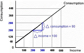
$ 0 $ 40 | | | | | 100 120 | | | | | 200 200 | | | | | 300 280 | | | | | 400 360 | | | | | 500 440 | | | | |
As expected, as the economy's GDP (income) increases, household
consumption increases. GDP and consumption are directly related. If
we graphed this consumption data we would get:
or
disposable income
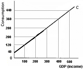
Notice that when income is equal to $ 0, there is still some consumption ($ 40 billion). this is called "autonomous consumption". It is consumption that is not related to income. Think about what a GDP of $ 0 represents. If GDP, or an economy's income, were equal to $0, this means that nothing was produced in this. If an economy does not produce a thing, would there still be some consumption? Yes, but how? they would consume goods that were saved from earlier periods. Of course, a GDP of $0 is a ridiculous concept, but there are two components to household consumption: (1) autonomous consumption that is not related to income, and (2) induced consumption or consumption that is directly related to income.
Now, to understand, and calculate, the multiplier, we need to complete the table.
First we need some simplifying assumptions to make our model easier to understand:
|
GDP |
= |
C |
+ |
I |
Given these assumptions we can calculate saving (S). With these assumptions there are only two things that consumers can do with their income, spend it (C) or save it (S). So:
|
income |
= |
C |
+ |
S |
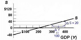
Therefore, we can calculate saving: Saving is a schedule which shows the amounts households plan to save (plan not to spend for consumer goods), at different levels of disposable income.
$ 0 $ 40 $ - 40 | | | | 100 120 - 20 | | | | 200 200 0 | | | | 300 280 20 | | | | 400 360 40 | | | | 500 440 60 | | | |
Notice that both consumption and saving is directly related to
income. When income increases both consumption and savings
increase.
(income)
Average Propensity to Consume (APC) and Average Propensity to Save (APS)
With this data we can calculate the APC and APS for each level of income.
APC is the fraction of the economy's total income that is spent (consumed) and APS is the fraction of total income that is saved.
|
C |
|
|
APC = |
-------- |
|
income |
|
S |
|
|
APS = |
-------- |
|
income |
When we calculate APC and APS we get:
$ 0 $ 40 $
- 40 100 120 - 20 1.2 - 0.2 | | 200 200 0 1.0 0 | | 300 280 20 0.93 .07 | | 400 360 40 0.90 .10 | | 500 440 60 0.88 .12 | |
(income)
Notice that for each level of income: APC + APS = 1. Given our assumptions there are only two things that consumers can do with their income: spend it or save it. If you add the fraction of the total income that is spent (APC) and the fraction of the total income that is saved (APS) we get all of our income, or 1.
Can you think of anything else that we can do with our income besides spend it or save it? Many students will answer "invest it". But what does investment mean in economics? Investment is the accumulation of capital. "Capital" is a manufactured resource. Therefore, "investment" occurs when a carpenter buys a hammer or if McDonald's builds a new restaurant. Putting money into the stock market is NOT investment, it is saving.
Marginal Propensity to Consume (MPC) and Marginal Propensity to Save (MPS)
To understand the multiplier effect we need to know what happens to ADDITIONAL, or MARGINAL, income.
Earlier we explained that the multiplier works "because an initial change in spending will cause an initial increase in GDP and it also becomes income to someone else. (If I buy a new car, people who built and sold that car earn income equal to the price of the car.) What will these people do with their additional income? Well, they will spend some and save some. " But HOW MUCH will they spend of this additional income and HOW MUCH will they save of this additional income? To know this we need to calculate the MPC and MPS.
With our consumption and savings data we can calculate the MPC and MPS for each level of income.
MPC is the fraction of the economy's additional income that is spent (consumed) and MPS is the fraction of additional income that is saved.
"Marginal" means "additional" or "extra"
|
change in C |
|
|
MPC = |
----------------- |
|
change in income |
|
change in S |
|
|
MPS = |
----------------- |
|
change in income |
To calculate MPC and MPS select two levels of GDP or income. For example if income increases from $0 to $100, then consumption increases from $40 to 120. Therefore if income increases from $0 to $100 then the change in income is $100 and the change in consumption is $80. MPC is then equal to 0.8.
|
|
|
||||
|
MPC = |
--------------- |
|
|
|
|
|
|
|
If you do the same thing for MPS you will get MPS = 0.2.
$ 0 $ 40 $
- 40 100 120 - 20 1.2 - 0.2 0.8 0.2 200 200 0 1.0 0 0.8 0.2 300 280 20 0.93 .07 0.8 0.2 400 360 40 0.90 .10 0.8 0.2 500 440 60 0.88 .12 0.8 0.2
Notice that for each level of income, MPC + MPS = 1. There are
two things that you can do with additional income: spend a
fraction (MPC) and save a fraction (MPS). If you add these fractions
together you will get 1.
(income)
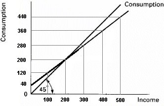
If you remember your 8th grade math you would recognize that our formula for MPC is actually the slope of the consumption graph.
|
|
|
||||
|
MPC = |
|
|
|
|
|
|
|
|
|
|
|
And the same is true for MPS:
|
|
|
One last item needs to be discussed: are MPC and MPS really constant? Note that in our table MPS equals 0.8 for all income levels and MPS equals 0.2. This means that if you get a raise (or additional income) of $1000 you would spend $800 of the raise (0.8 x 1000 = $800) and you would save $200 of it (0.2 x $1000 = $200). But is the fraction of additional income that is spent and saved really constant for all levels of income?
Let's assume that I am going to give two families $10,000 in additional income. So I go to the housing projects in Chicago and find a poor family and give them $10,000 and I fly to the state of Washington and find Bill Gates (probably the richest person in the world) and give him $10,000. Would they both spend and save the same fraction of this additional income?
No, the poor family would most likely spend the whole $10,000 and Bill Gates would probably spend nothing of the addition income. So the MPC of the poor family would be very high, or equal to 1, and the MPC of Bill Gates would be very low, or equal to 0. So as GDP or income increases, MPC should get smaller, or decrease, and MPS increases. This means the slope of the consumption graph should get smaller (flattens out) as GDP increases.
We will assume that the MPC is constant in this course. That way we can use straight line consumption graphs and we can find the MPC by finding its slope.
If you cut taxes on lower income people and raise taxes on higher income people, what effect, if any, will it have on aggregate demand?
"Eliminate payroll taxes to improve economy"Marketplace commentator Robert Reich thinks that reducing payroll taxes will get consumers to start spending again, which will help get the economy moving again.
Text / Link to audio:
http://marketplace.publicradio.org/display/web/2010/08/25/pm-reich-eliminate-payroll-taxes-to-improve-economy/
To keep things simple let's assume that we have an economy with only consumers and businesses. Therefore:
GDP = C + Ig
Now let's assume that in this economy (let's say that it represents the Chicago area) a new stadium worth $20 million is built. What is the total impact of this investment on the economy?
Well, if GDP is the total market value of all final goods and
services produced in an economy in one year , then building this $20
million stadium will increase GDP initially by $20.
GDP = Income = C + I + 20 + 20
![]()
But when $20 is spent (and therefore $20 is produced) $20 is also earned as income to those who did the producing. so income also increases by $20. What do these people do with this additional income? Well, they spend a part and save a part. How much do they spend and save? What concept tells us the change in consumption that results from additional income? . . MPC !
|
|
|
|
MPC = |
--------------- |
|
|
Let's use the MPC that we calculated above, so MPC = 0.8
So if incomes go up by $20, consumption will increase by $16
Change in C = (MPC) x (change in income)
Change in C = (0.8) x ($20) = $16 (we call this a induced
consumption)
and the change in S = $4
Change in S = (MPS) x (change in income)
Change in S = (0.2) x ($20) = $4
So we get the following
GDP = Income = C + I + 20 + 20 + 16 +16 + 4
![]()
![]()
![]()
GDP has gone up by an additional $16, therefore so has income. What will they do with this additional income? They will spend 80% (MPC=0.8) of it and save 20% (MPS=0.2).
So we get the following:
GDP = Income = C + I + 20 + 20 + 16 +16 + 4 + 12.8 + 12.8 + 3.2
![]()
![]()
![]()
![]()
![]()
And again, GDP has increased. This time by $12.8 and so has income, part of which will be spent and part saved. So consumption and GDP increase by $10.24 (0.8 x 12.8) and saving increases by 2.56 (0.2 x 12.8).
GDP = Income = C + I + 20 + 20 + 16 +16 + 4 + 12.8 + 12.8 + 3.2 + 10.24 + 10.24 + 2.56
![]()
![]()
![]()
![]()
![]()
![]()
![]()
This process will go on and on. When will it stop? If we add up all that has been saved and it equals 20, ( 4 + 3.2 + 2.56 + ...+...+...+...= 20) then there is nothing left to spend and the process stops. If you do this you will get the following total changes:
GDP = Income = C + I + 20 + 20 + 16 +16 + 4 + 12.8 + 12.8 + 3.2 + 10.24 + 10.24 + 2.56 total change total change total change + 100 + 80 + 20 + 20
![]()
![]()
![]()
![]()
![]()
![]()
![]()
![]()
![]()
![]()
![]()
So with an initial increase in spending of $20, GDP increases by $100.
The most important formula for you to learn is:
|
change in GDP |
= |
initial change in spending |
|
multiplier |
So using our data we get:
change in GDP initial change in spending multiplier
The size of the multiplier depends on how much of additional income is NOT spent. In our example the MPS is .2, so 20% of additional income is not spent, but rather it is saved. The multiplier then is:
|
|
|
||||
|
Multiplier = |
-------- |
= |
-------- |
= |
5 |
|
MPS |
0.2 |
Graphically -- how does the multiplier work?
THIS IS IMPORTANT!
(Be sure you understand table 10-3 and Figure 10.8 in the textbook.)Assume: MPC = .8, and I increases by $20 billion
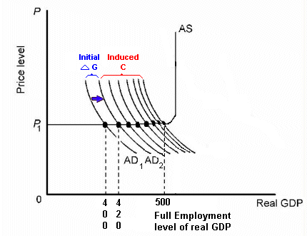
So initially, since I increased by $20, the AD curve shifts to the left by $20 (see graph below).
But since GDP has increase by $20 (see graph above) income has also increased by $20. What will people do with this additional income?
Spend some (MPC) and save some (MPS). The extra spending is consumption (C) and this shifts the AD curve further to the right. But, again, additional spending becomes additional income for someone else, part of which would be spend and part saved. The part spent shifts the AD curve some more. This process will continue until all of the initial investment ($20) is saved
The multiplier and marginal propensities (slopes)
1
a. multiplier =
-------
MPS
1
b. multiplier =
------------
1 - MPC
A larger MPC (or smaller MPS) has a larger multiplier
IF the MPS is:
Then the multiplier is:
.1 10 .2 5 .75 4 .67 3 .5 2 In other words, the more that is NOT SPENT, the smaller is the additional spending that results, and the multiplier is smaller.
The Complex Multiplier (or the
ACTUAL multiplier)
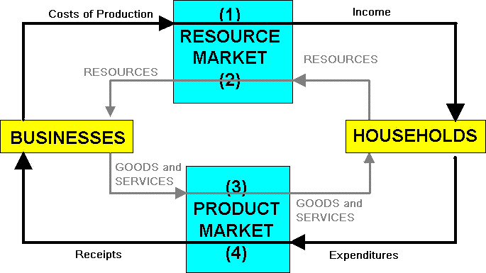
We can see from the circular flow diagram of chapter 1 that income becomes expenditure (or AD).But not all income becomes spending. What ELSE can you do with your Disposable Income (DI) besides spend it?
- You can save it
- saving is a "leakage" from the income = expenditure stream
- this creates the simple multiplier we learned above
- But you can also use disposable income to pay taxes. This is another "leakage" from the income=expenditure stream.
- Also, you can also spend it on imports. This is another "leakage" from the income = expenditure stream, because this spending on imports becomes income for people in the foreign country.
- So not all increases in income become additional spending.
- How does this affect the size of the multiplier?
DI
C
AD
Leakages
Injections
S I T G M X If there are more leakages, the multiplier is smaller
1 actual multiplier =
------------- leakages
1 complex multiplier =
------------- MPS + MPT + MPM
- Where MPS is the marginal propensity to save or the fraction of additional income that is saved and so it doesn't become income for someone else.
MPT would be the "marginal propensity to tax" or the fraction of additional income that is paid in taxes and so it doesn't become income for someone else.
MPM would be the "marginal propensity to import" or the faction of additional income that is spent on imports and so it doesn't become income for someone else in the country where it was spent.
The Complex (or ACTUAL) Multiplier is SMALLER than the Simple Multiplier because there are more leakages and less induced consumption.
We learned in the AS/AD chapter that the nonincome determinants of consumption and saving can cause people to spend or save more or less at various income levels, although the level of income is the basic determinant. The following are the determinants of consumption (and AD) that we studied in chapter 12. See Figure 10.4
1 Wealth: An increase in wealth shifts the consumption schedule up, saving schedule down and AD to the right In recent years major fluctuations in stock market values have increased the importance of this wealth effect. A "reverse wealth effect" occurred in 2000 and 2001, when stock prices fell dramatically. Consider This … What Wealth Effect?2. Expectations: Changes in expected future prices or wealth can affect consumption spending and AD today.
3. Real interest rates: Declining interest rates increase the incentive to borrow and consume, reduce the incentive to save, and increase AD. Because many household expenditures are not interest sensitive - the light bill, groceries, etc. - the effect of interest rate changes on consumption spending are modest (but interest rates do have a significant effect on investment).
4. Household debt: Lower debt levels shift consumption schedule up, saving schedule down, and increases AD.
Other important considerations: See Figure 10.4.
1. Macroeconomic models focus on real domestic output (real GDP) more than on disposable income. Figure 10.4 reflects this change in the labeling of the horizontal axis.2. Changes along schedules: Movement from one point to another on a given schedule is called a change in the amount consumed; a shift in the schedule is called a change in consumption schedule, and is caused by nonincome determinants of consumption
3. Schedule shifts: Consumption and saving schedules will always shift in opposite directions unless a shift is caused by a tax change.
4. Taxation: Lower taxes will shift both schedules up since taxation affects both spending and saving, and vice versa for higher taxes.
5. Stability: Economists believe that consumption and saving schedules are generally stable unless deliberately shifted by government action.
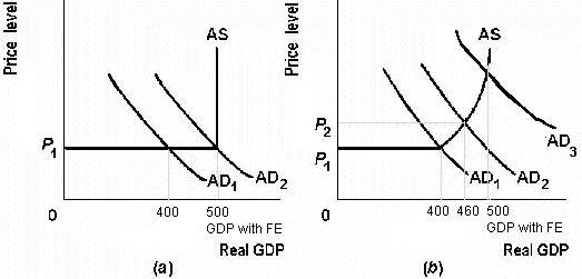
The Multiplier with Changes in the Price Level
We have been assuming that the price level does not change as AD increases (see graph).
But in the real world as GDP increases and approaches the full employment level of output the price level will begin to rise and resource costs increase.
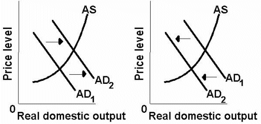
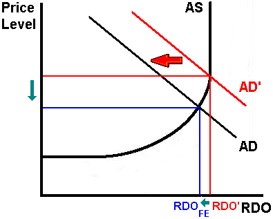
How does this inflation, which results from an increase in AD, affect the size of the multiplier? Or, what happens to the change in government spending needed to achieve full employment if we allow for inflation? Without inflation, and with an MPC of 0.8, if we increase government spending by $20 then GDP will increase by $100 because the multiplier is 5. This will shift AD from AD1 to AD2 in both graphs above. In graph (a) without inflation the equilibrium GDP increases from $400 to $500. But in graph (b) with inflation the same horizontal shift in AD increases GDP from $400 to only $460. From the same change in government spending ($20) GDP increases a small amount. With inflation the multiplier is smaller.
To calculate the multiplier with changes in the price level you need to know the initial change in spending ($20 in our example) and the resulting total change in GDP ($60 from graph b above).
change in GDP = initial change in spending x multiplier + $60 = + $20 x ? + $60 = + $20 x 3
Remember, the term "investment" consists of spending on new plants, capital equipment, machinery, inventories, construction, etc. It does NOT mean "investing" in the stock market or buying bonds. Buying stocks and bonds is SAVING (not spending).How much businesses spend on capital depends on (1) what they expect to make from it and (2) the cost of borrowing to pay for it. What they expect to make is called the "expected rate of return" and what they have to spend to borrow to pay for the capital is the interest rate they pay for the loan.
Expected rate of return is found by comparing the expected economic profit (total revenue minus total cost) to cost of investment to get expected rate of return. The text's example gives $100 expected profit on a $1000 investment, for a 10% expected rate of return. Thus, the business would not want to pay more than 10% interest rate on investment. Remember that the expected rate of return is not a guaranteed rate of return. Investment carries risk.
The real interest rate, i (nominal rate corrected for expected inflation), determines the cost of investment.
1. The interest rate represents either the cost of borrowed funds or the opportunity cost of investing your own funds, which is income you won't get.2. If real interest rate exceeds the expected rate of return, the investment should not be made.
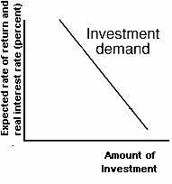
Investment demand schedule, or curve, shows an inverse relationship between the interest rate and amount of investment.
1. As long as expected return exceeds interest rate, the investment is expected to be profitable (see the Table 10.2 example).2. Key Graph 1.5 shows the relationship when the investment rule is followed. Fewer projects are expected to provide high return, so less will be invested if interest rates are high.
In chapter 10 we discussed the determinants of Investment, which are determinants of Aggregate Demand. Shifts in investment demand (Figure 10.6) occur when any determinant apart from the interest rate changes. This also shifts AD.
1. Greater expected returns create more investment demand; shift curve to right. The reverse causes a leftward shift.2. Changes in expected returns result because:
a. Acquisition, maintenance, and operating costs of capital goods may change. Higher costs lower the expected return.b. Business taxes may change. Increased taxes lower the expected return.
c. Technology may change. Technological change often involves lower costs, which would increase expected returns.
d. Stock of capital goods on hand will affect new investment. If there is abundant idle capital on hand because of weak demand or recent investment, new investments would be less profitable.
e. Expectations about future economic and political conditions, both in the aggregate and in certain specific markets, can change the view of expected profits
Unlike consumption and saving, investment is a very unstable type of spending; I is more volatile than GDP (See Figure 8.7). Investment is unstable because:
- Capital goods are durable, so spending can be postponed or not. This is unpredictable.
- Innovation occurs irregularly.
- Profits vary considerably.
- Expectations can be easily changed.
Be sure to read "LAST WORD: Squaring the Economic Circle" in the textbook. It contains a humorous example of how the multiplier works. Furthermore it does a good job explaining how a small DECREASE in spending will result in a big decrease in overall spending and in GDP. Here is a summary: