The textbook and the online video lectures are written by
different authors and sometimes (often?) different economic authors
use different terminology or different approaches to discuss the same
concept. This webpage will help you see the connections between our
textbook and the online video lectures.
Also, this webpage will allow me to add some of my own comments
and explanations. All of my comments begin with "ME".
You should refer to this page when watching the videos. Don't
forget the quizzes (Thinkwell Exercises), transcripts, and lecture
notes that accompany most of the video lectures. These can be very
helpful.
Notes from the Video
Lectures
Unit 1: ECONOMICS and GLOBALIZATION
- 1a - Introduction to the
Course
- 1b - What is Economics and the
5Es
- 1c - Production Possibilities (PPC)
and BCA
- 2a - Economic Systems and
Globalization
- 2b - Role of Government and
Government Finance
- 3a - Demand
- 3b - Supply
- 3c - Market Equilibrium and
Efficiency
- 20a -Why we Trade: Comparative
Advantage
- 20b - International Trade
|
Unit 2: INTRO. TO MACROECONOMICS
- 12a - Introduction to
Macroeconomics and AD
- 12b - AS and Equilibrium: Using
AD/AS
- 12c - AS/AD in the Long Run
- 9a - Unemployment (UE)
- 9b - Inflation (IN)
- 7a - Measuring the Economy:
GDP
- 8a - Economic Growth (EG)
- 22Wa - Economic Growth in the
LDCs
|
Unit 3: MACROECONOMIC POLICY
MONETARY POLICY
- 14a - Money, Money Market, and the
Fed
- 15a - How Banks Create Money
- 16a - Monetary Policy (MP)
- 16b - Other Monetary Policy
Issues
FISCAL POLICY
- 10a - The Spending Multiplier
- 13a - Fiscal Policy
- 13b - Other FP Issues and the
Public Debt
|
Unit 1: ECONOMICS and
GLOBALIZATION
|
LESSON 1a - Introduction to the Course
- WHAT IS ECONOMICS: THE STUDY OF SCARCITY
- REVIEW OF GRAPHING CONCEPTS
1.1.1 (6:35) Scarcity - Defining
Economics
- Outline:
- what is economics?
- opportunity costs
- the big picture: economic models
- definition of economics: rational choice under conditions of
scarcity
- what is scarcity?
- ME: limited resources vs. unlimited human wants
- what is rational choice? = self interest, comparing costs and
benefits to maximize satisfaction = calculated self interest
- ME: Our textbook calls this "Benefit Cost Analysis" or MB =
MC
- ME: we will be using this a lot this semester
- ME: whenever you get a chance, pay close attention to
"rational choice" or "Benefit Cost Analysis". You will need to
know it.
- calculated self interested people operating under conditions
of scarcity = economics
- opportunity cost
- no such thing as a free lunch
- we can make economic models about almost anything
- ME: what I like about economics is it's use of models
- ME: I think teaching students the benefits of using models
and how to use models is one of the most important goals if
this course
- ME: most models in economics involve the use of graphs
1.1.2 (13:20) What Economists Do
- Outline:
- scientific method
- ask questions
- produce models
- form hypotheses
- where to find economists
- normative vs. positive economics
- the STUDY of economics = social science = uses the scientific
method = asking a question = why?
- what to produce?
- how will it be produced?
- who is going to get what is produced?
- building a scientific model = map = the model (map) that you
use depends on the question being asked providing only the
information needed to answer the question
- hypotheses = predictions on how the world works = can be
tested with data
- building relationships between variables by ignoring variables
that do not matter to the questions being investigated
- ME: models are SIMPLIFICATIONS of reality
- ME add more: GENERALIZATION
- ABSTRACTION
- ask a question
- isolate related variables and build model
- come up with hypotheses that you can test with data
- ceteris paribus: holding all other factors constant to
help see relationships between just two variables
- Positive economics vs normative economics
- positive: what IS happening? what will happen, predictions,
and descriptions how world does work
- normative: what SHOULD we do? judgments What is good? how
world should work
1.1.3 (11:21) Microeconomics and
Macroeconomics
- Outline:
- microeconomics vs. macroeconomics
- players in the economy
- nominal vs. real variables
- microeconomics vs macroeconomics
- individuals vs aggregate, biology analogy: cell vs. whole
organism
- macro: study of the economy as an organism, study of the
overall economy
- micro: how the cell works; individual parts of the
economy
- MICRO: the way a particular household responds to changes in
incentives
- ignores money, relative prices rather than monetary
prices
- MACRO: money is the life blood of the macroeconomic organism
- money carries things through the system,
- difference: individual decision making vs. the whole
organism
- money is more or less ignored in micro vs. money is important
in macro
- the four major players: households, businesses, government,
foreigners (net exports) and how they are studied in micro vs.
macro
- "real" values are measured in terms of physical goods and
services
- "nominal" values are measured in dollar terms, money; $1.25
(nominal) vs a real cup of coffee (real)
REVIEW OF GRAPHING
CONCEPTS
1.2.1
(9:50) Using Graphs to Understand Direct Relationships
- Outline
- How do graphs work?
- About this graph
- How do graphs work
- economists use graphs to represent the relationship between
two variables (sometimes three) in a two-dimensional space
- Example: the relationship between consumption and income
- income on horizontal axis and consumption on the
vertical axis
- ALWAYS LABEL THE AXES
- calibrate the axis with numbers
- put data points on the graph; every point on a graph
represents two numbers
- (horizontal, vertical); (x,y); (30,40)
- About this graph
- the x-axis is horizontal
- the y-axis is vertical
- a scatter diagram (or scatter plot) is a collection
of points on a graph showing the observed relationship between
two variables
- ME: even though Tomlinson just puts a bunch of points on
the graph, each one of them should have been actual observed
data; you can't just make up points on a graph
- ME: most people seem to use the terms "scatter diagram" and
"scatter plot" TO MEAN THE SAME THING
- "fitting" a line to the scatter plot to show the
relationship between the two variables
- on the scatter plot it looks like when income increases
consumption also increases
- x and y are directly related when if x increases
then y increases, or if x decreases then y decreases; a
direct relationship is also called a positive
relationship
- "fitting a line to a scatter plot means that you draw a
straight line that is as close to all the dots as
possible
- an upward sloping (from left to right) line on a graph
indicates a direct relationship
- an upward sloping line will have a positive slope
(we will discuss the idea of slope more later)
- economists will first notice general relationships between
data points like the positive, or direct. relationship between
income and household consumption
1.2.2
(9:57) Plotting A Linear Relationship Between Two Variables
- Outline
- Creating the demand curve
- The demand curve
- Formula for the demand curve
- The slope describes the consumer's behavior when price
changes
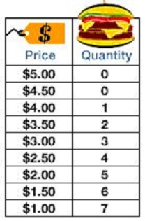
- Creating the demand curve
- look at the data and determine the relationship between the
two variables
- draw, LABEL, and calibrate the axes ("calibrate" means put
numbers along the axes)
- the "origin" is the point where the x and y axes
intersect
- plot the data on the graph
- connect the points to draw the demand curve
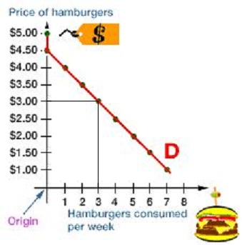
- The demand curve
- the demand curve shows the relationship between the price
of a good and he quantity a consumer wants to buy
- ME:
- note that as the price of hamburgers goes down then Bob
will buy more hamburgers
- this represents an inverse, or negative,
relationship between price and quantity of hamburgers
purchased
- an downward sloping (from left to right) line on a graph
indicates an inverse relationship
- an downward sloping line will have a negative
slope (we will discuss the idea of slope more
later)
- Formula for the demand curve
ME: We will not do this.
- y = a + bx
- y = the vertical axis variable (Price)
- a = the y-intercept
- b = slope
- x = the horizontal axis variable (Quantity)
- in our example:
- Price = $4.50 - $0.50 * Quantity
- P=4.50 -.5Q
- The slope describes the consumer's behavior when price changes
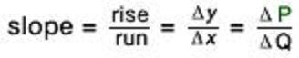
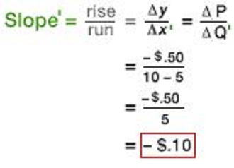
- b = slope = rise/run =
 y/x
= change in price / change in quantity = P/Q
y/x
= change in price / change in quantity = P/Q
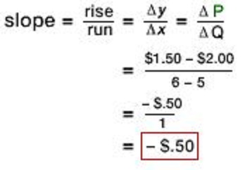
- if the price of hamburgers decrease by $0.50 then Bob will
buy one more hamburger
- b = P/Q
- slope = -$0.50 / 1 = -0.50
- slope is negative indicating the inverse relationship
(or that have to DECREASE the prise to get Bob to
INCREASE the quantity that he will buy)
- ""
means "change"
- ME:
- So, if you know the y-intercept and the slope
of a straight line you can find all of the possible
values for the two variables
- we know that a=4.50 and b=-.50, then
- if the price is $3.00 how many burgers will Bob
buy?
- first, write down the information that you
have:
- price = y = 3.00
- y-intercept = a = 4.50
- slope = b = -.50
- then, write down the formula:
- y = a + bx
- Price = y-intercept + slope times the
quantity
- now, plug the data into the formula
- finally, you can you solve for Q
- subtract 4.50 from each side:
- 3.00 - 4.50 = 4.50 + -50Q - 4.50
- -1.50- = -50 * Q
- then divide each side by -50:
- -1/50/-50 = (-.50Q)/.50
- -1.50/.50 = Q
- 3 = Q;
- if you look at the graph or the table you
can see that we got it right; when the price
was $3.00, Bob bought 3 hamburgers
|
|
1.2.3
(8:42) Changing the Intercept of a Linear Function
- Outline
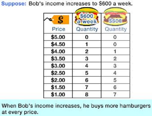
- What happens if we change Bob's income?
- Raising Income
- Lowering income
- Summary
- What happens to the relationship between price and quantity if
we change Bob's income?
- Raising Income
- if Bob gets a higher income we can expect that he will
change his behavior; he will probably buy more hamburgers
- on the demand table we can see that at the same prices, Bob
will buy more hamburgers
- on the graph, with the higher income the y-intercept has
increased and the demand curve has moves to the right
- the slope is still the same so we still have the same
negative relationship, but now with higher quantities
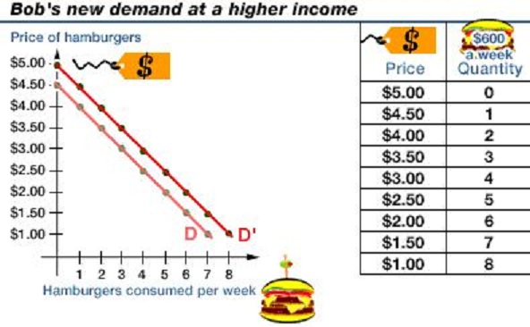
- formula for the new demand if Bob's income increases: P =
5.00 -.50Q
- the curve has shifted to the right
- Lowering income
- we can do the same thing for a lower income causing the
curve to shift to the left
- this will decrease the y-intercept (but keep the slope the
same)
- formula for the demand with a lower income: P = 4.00
-.50Q
- the curve has shifted to the left and the slope stays the
same
- Summary
- a change in income will result in a parallel shift of the
demand curve
1.2.4 (7:28) Understanding the Slope of a
Linear Function
- Outline
- What does the slope of a demand curve indicate?
- Units and Slope
- What does the slope of a demand curve indicate?
- the sensitivity of Bob's demand for hamburgers to changes
in the price
- or, what happens to the number of hamburgers that Bob buys
each week when the price changes?
- this will help us understand how economists think about the
slope of a line
-
- in our original example we saw that when the price of
hamburgers fell by $0.50 then Bob would buy one more hamburger
a week
- so if the price goes down from $2.00 to $1.50
- What if the slope of the demand curve changes?; What if Bob
has a different relationship between price and quantity?
- if price = $2.00 then he would buy 5 hamburgers and if
price = $1.50 he would buy 10 hamburgers
- result: and new demand curve with a different slope; a
flatter slope; and smaller slope
- now Bob is more sensitive to a change in price; now, a
$0.50 decrease in price causes Bob to buy a lot more (5)
hamburgers; or when the price decreases by just a dime
($0.10) he will buy one more hamburger
- the slope of curves indicates the sensitivity of one
variable to changes in another
- Units and Slope
- Warning: the slopes of the curves depends completely upon
the unit in which the variables are measured
- here we were measuring the price of hamburgers in
dollars ($4.00, $3.50, $3.00, etc)
- but the slopes would change if we measured the prices in
cents (400 cents, 350 cents, 300 cents, etc)
- so if we change the way we measure the price, then the
slopes will change
- the same thing happens if we change the way that we
measure burgers (boxes of burger, or half burgers, etc)
- so if we want to measure the sensitivity of one variable to
changes in another we can't use slope since slopes can change
just because we change the units, even though the sensitivity
is the same
- therefore economists use something class
"elasticity" to measure sensitivity
- the price elasticity of demand is the percentage
change in the quantity demanded that results from a percentage
change in price
- since elasticity uses percentage changes, is doesn't matter
whether we measure the price of hamburgers in dollars or in
cents, the elasticity (sensitivity) will be the same
OPTIONAL: SIMPLE MATH,
ALGEBRA AND GEOMETRY FOR ECONOMICS STUDENTS
How to Multiply and Divide Fractions in
Algebra for Dummies (YouTube fordummies 1:50)
http://www.youtube.com/watch?v=B7MtFQW7i_I
- 2/5 x 3/7
- 2/3 x 3/8
- 2/3 x 3/7
- 1/3 ÷ 4/5
Simple Equations (11:06)
http://www.khanacademy.org/math/algebra/solving-linear-equations-and-inequalities/v/simple-equations
- 7x = 14 (very elementary)
- 3x = 15 (6:00 is a good place to start)
- 2y + 4y = 18
Solving One-Step Equations (1:54)
http://www.khanacademy.org/math/algebra/solving-linear-equations-and-inequalities/v/solving-one-step-equations
- a + 5 = 54; solve for a and check your solution
Solving One-Step Equations 2 (2:23)
http://www.khanacademy.org/math/algebra/solving-linear-equations-and-inequalities/basic-equation-practice/v/solving-one-step-equations-2
- x/3 = 14; solve for x and check your solution
Solving Ax + B = C (8:41)
http://www.khanacademy.org/math/algebra/solving-linear-equations-and-inequalities/basic-equation-practice/v/equations-2
- 3x + 5 = 17 (very elementary)
- 7x - 2 = -10 (starting at 5:20)
Area and Perimeter (12:20)
http://www.khanacademy.org/math/geometry/basic-geometry/v/area-and-perimeter
- area of a square
 (very elementary; he does make an adding error!)
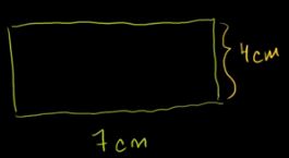
- area of a rectangle (begins at 5:00)
- area of a right triangle (begins at 6:44)
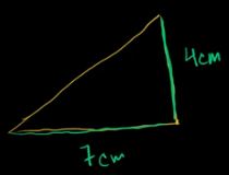
- area of a triangle (begins at 10:06)
LESSON 1b - The 5Es of Economics
LESSON 1c -Production Possibilities (PPC) and
Benefit Cost Analysis (BCA)
1.4.1 (24:46) Understanding the Concept of
Production Possibilities Frontiers - 1c
- Outline:
- scarcity and efficiency
- production possibilities table
- production possibilities curve
- calculating opportunity costs
- production possibilities curve - PPC (also called the
production possibilities frontier - PPF) and scarcity
- ME: This is our second model or graph
- first: discuss efficiency: doing the best with what you have =
getting the most you can from what you have
- efficient behavior is to produce the most wheat with a given
quantity of rice
- only two goods produced - what is the optimal output of wheat
and rice this economy can produce
- need to know what resources and what technology is
available
- ME: our textbook lists 5 assumptions of the production
possibilities curve:
- fixed resources
- fixed technology
- productive efficiency
- full employment
- only two goods being produced
- technique vs. technology
- technique = a particular combination of inputs
- technology = all the possible combination of inputs = a
catalog of all the things an economy knows how to do
- improved technology = more output with less input
- production possibilities table : every combination is an
"efficient" combination that can be produced = maximum amount that
can be produced
- ME: Note how Professor Tomlinson is moving the "best suited"
resources first to the production of rice; this allows a large
increase of rice production with only a small loss of wheat
production
- "efficient combination of resources" means that we are
producing the maximum quantities possible
- the production possibilities curve (PPC) is also called the
production possibilities frontier (PPF)
- first label the axes
- then calibrate the axes
- now plot the points that represent the possible combinations
of wheat and rice that can be produced
- ME: any point on a graph represents two numbers; don't get
scared, all we are doing is looking at only TWO NUMBERS for each
point on the graph
- then connect the dots to draw the graph
- NOTE: the shape of the PPC
- PPC is a collection of points representing the maximum
combinations of output an economy can produce given that economy's
technology and resource endowment (amounts)
- What the PPC represents:
- points (quantities of wheat and rice) outside of the curve
are not attainable (ME: such quantities are IMPOSSIBLE
with the given technology and resources THEREFORE WE MUST
MAKE CHOICES)
- points within the PPC are possible but are less than the
maximum possible. If there is inefficiency or unemployment then
less than the maximum possible will be produced and the economy
will be at a point within their PPC
- a point within the curve (i.e. less output) is also what
happens if there are UNEMPLOYED resources
- ME: when Tomlinson is discussing using wet land for
wheat and dry land for rice he is talking about
PRODUCTIVE INEFFICIENCY - not using resources
where they are best suited (from the online 5Es lecture). He
calls this the "underemployment of resources". I call this
"productive inefficiency" (5Es)
- OPPORTUNITY COST = downward sloping PPC; wheat is
the opportunity cost of rice: Why?
- CALCULATING THE OPPORTUNITY COST. Know how to do
this!
- opportunity cost = change in wheat/change in rice
- opportunity cost is the slope of the line connecting the
two points
- Why does the opportunity cost (slope) of producing rice
increase as more rice is produced?
- i.e. why does the PPC get steeper as we increase the
quantity of rice?
- shape of PPC is CONCAVE (bowed out)
- ME: our textbook calls this the "Law of Increasing
Costs"
- WHY?
- Because not all resources are the same. Some are
better for producing rice and others are better suited to
producing wheat
- this causes the opportunity costs to increase as we
produce more rice
- i.e. this causes the shape of the PPC to be concave
(bowed out)
- SUMMARY: 4 things we can see in the PPC
- some combinations are impossible so therefore there is
scarcity AND we must then make choices
- unemployed resources and productive inefficiency causes
less than the maximum level of production
- there are opportunity costs
- the PPC is concave representing increasing opportunity
costs because not all resources are the same, some are better
suited to producing rice and others are better suited to
producing wheat
- ME: from our yellow pages
- The Production Possibilities Curve can be used to
illustrate several important economic concepts:
- we must make choices
- choices have opportunity costs
- the law of increasing costs
- the effect of unemployment
- the effect of productive inefficiency
- the effect of economic growth
- how present choices affect future possibilities
- it does NOT show the optimum product mix
(allocative efficiency)
- Later we'll use the MB=MC analysis to do this (see
figure 1.3 [p. 13] of your textbook)
1.4.2 (10:10) Understanding How a Change in
Technology or Resources Affects the PPC - 1c
- Outline:
- production possibilities curve
- outward shift (ME: called "economic growth")
- individual product shift
- inward shift
- summary
- What happens if there is a change in technology or amount of
resources? PPC will shift out
- What is the difference between an movement along an existing
PPC and shifting the curve to a new curve?
- If BETTER TECHNOLOGY for rice and wheat production is
discovered, the curve will shift outward representing that MORE
can be produced i.e the quantities on the production possibilities
table get larger
- What if we get MORE RESOURCES like more labor? Answer: PPC
shifts outward
- ME: our textbook calls this "economic growth".; Definition:
and increase in the ABILITY to produce caused by getting more
resources, getting better resources, or getting better
technology
- What if we ONLY get better technology for wheat but not for
rice? A "skewed" shift outward of the PPC.
- What if there is a change in climate hurting the production of
wheat but helping the production of rice? Again, a "skewed" shift
outward of the PPC.
- What if there are FEWER RESOURCES? The PPC will shift
inwards
- ME: there is a big difference between moving from a point on
the curve to moving to a point inside the curve AND the whole
curve shifting inward
- moving from a point on the curve to to a point inside the
curve is caused by not using all available resources
(unemployment) or productive inefficiency. If this happens we
still CAN produce the same quantities as before, but we are
just not achieving our potential; our possible production did
not change
- the whole curve shifting inward is caused by there being
fewer resources than before (depletion) and now the maximum
that can be produced is less; out potential has decreased
- QUESTION: Which combination of wheat or rice is
preferred? ME: Which is the allocatively efficient quantity?
ANSWER:"We have no idea." The PPC is not designed to tell us what
we want. It is designed to tell us what is possible. We will have
a different model in a later chapter to tell us what we want -
what quantities will maximize our satisfaction (allocative
efficiency)
- ME: when Tomlinson is discussing "efficiency" he seems
to be discussing only PRODUCTIVE EFFICIENCY. Now would be a good
time to re-read the 5Es lecture: http://www.harpercollege.edu/mhealy/eco212i/lectures/ch1-18.htm
MAKING CHOICES: THE ECONOMIC
WAY OF THINKING -- BENEFIT-COST ANALYSIS (also called Marginal
Analysis or Cost-Benefit Analysis)
Thinking at the Margin (LearnLiberty 4:32) -
1c
http://www.youtube.com/watch?v=tMhdTn-5fu8
- ME: "marginal" means "extra" or "additional"
- individuals make choices based on comparisons at the
margin
- when wanting to make the best choice we compare the
options
- "thinking at the margin" means we look at the next option
- why are diamonds more expensive than water?
- because when you compare the value of an extra unit of
water (the marginal unit) with the extra unit of diamonds
- we make choices at the margin all the time,
- also businesses make decisions at thre margin, decisions like:
- should we hire an extra employee?
- we compare the extra cost of that employee, called the
marginal cost (MC)
- with the extra benefits that we will get from that
worker -- i.e. the marginal benefit (MB)
Incentives and Marginal Analysis
(MrHurdleHistory 8:54) - 1c
http://www.youtube.com/watch?v=dN9KyDCur2Y
- to make the best decision:
- select all options where the MB > MC (marginal benefits
are greater then the marginal costs OR extra benefits are
greater than the extra costs)
- up to where the MB = MC
- but never where the MB < MC
- the BEST CHOICE is always where MB =MC
- changes in MB and MC: [ME: KNOW THIS]
- if the MB increase, people will do more
- if the MB decrease then people will do less
- if the MC increase then people will do less
- if the MC decrease then people will do more
LESSON 2a - Economic Systems and Globalization
(Structural Adjustment)
- ECONOMIC SYSTEMS
- TRANSITION ECONOMIES
- GLOBALIZATION
ECONOMIC SYSTEMS
1.1.4 (10:50) An Overview of Economic Systems -
2a
- Outline
- Three Economic Questions
- Pure Laissez-faire economic system
- Centrally-planned economic system
- Mixed economic systems
- Every economic system must answer three questions
- What will be produced
- How will it be produced
- Who will get what is produced
- ME: the textbook lists five fundamental questions
- What goods and services will be produced?
- How will the goods and services be produced?
- Who will get the goods and services?
- How will the system accommodate change?
- How will the system promote progress?
- Pure Laissez-faire economic system - One EXTREME
- ME: This is what most people call a "market economy" or
"capitalism"
- "Laissez-faire" is French for "leave us alone" or "let us
do"
- everyone makes their own decisions
- prices arise in a market and these prices provide
incentives to guide resources
- the role of prices is very important in coordinating the
use of resources
- law of the jungle
- maximum individual freedom
- all people respond according to what they perceive is best
for them
- problems:
- end result might end up not being best fit society as a
whole
- examples of when the end result may be bad: (1)
standing up at a football game, (2) litter, (3) when
prices are not available to guide decisions like for
clean air
- monopolies may form
- Centrally Planned Economy - the other EXTREME
- ME: called a "command economy" inour textbook; sometimes
calle "socialism" or even "communism"
- central idea: a wise central planner make all the decisions
of when recourses would be used and how to generate wealth for
society
- Problems - where does the central planner get the
information to make good decision and how do they get each
resource to do what is assigned?
- via less freedom or monetary incentives?
- central planner does not have all the information
needed
- how do you keep the central planner from abusing their
power and work for the best interest of the society rather
than do what is best for themselves?
- Show which extreme view is better?
- In the real world all economic systems are MIXED
SYSTEMS including parts of laissez faire and parts of central
planning
- US: mostly laissez-faire with some central planning
- China: a lot of central planning and some
laissez-faire
- The role of the government in these mixed systems then is to
regulate the mix of these two extremes, some allow more
laissez-faire and some do more central planning
- a spectrum or continuum of mixed economic systems
Power of the Market (LibertyPen 1:14) -
2a
http://www.youtube.com/watch?v=4FHxpoQqPTU
- Milton Friedman (July 31, 1912 November 16, 2006) was an
American economist, statistician, and author who taught at the
University of Chicago for more than three decades. He was a
recipient of the Nobel Prize in Economics
- the invisible hand of capitalism -- what is it? ME: KNOW
THIS!
1.1.5 Case
Study: The Work of Adam Smith 8:57
- History of Adam Smith
- Important works and philosphies
- Self interest and common wealth
- Important works and philosophies
- THE THEORY OF MORAL SENTIMENTS
- human nature is compassionate and cooperative
- this makes us capable of producing great wealth
- THE WEALTH OF NATIONS
- the invisible hand of capitalism
- the important role of self interest
- self interest is not selfishness
- the result of pursuing your own self interest is an
increase in the wealth of society like an invisible hand is
guiding us to do not just what is good for us but what is
also good for all.
- Self interest and common wealth
- common wealth is accumulated by assessing your strengths
and where you can make a profit
- division of labor (the pin factory)
- benefits: efficient (more produced)
- Problems: monotonous
- Concerns:
- pollution
- monopolies (ME: lack of competition = inefficient)
- lack of information and the breakdown of trust
- the market does not always help the poor (ME:
inequity)
- damaging the human spirit by the division of labor
- Summary
- Smith believed in the free market (laizzez-faire) and
free trade to increase wealth
- but it is not completely clear whether is is for a
laissez-faire economy or a more active role for
government
- Maybe he is challenging us to justify government
intervention in the economy
- ME: we will look at the role of government in lesson 2b;
whenever the government is involved in the economy we should
ask WHY?
TRANSITION ECONOMIES
17.5.1
Centrally
Planned Economies 10:57
- Achieving specialization of trade through central
planning
- Problems with central planning
- Roles of the price mechanism
- Introduction:
- Adam Smith:a laissez faire market economy produces wealth
through people acting in their own self interest therefore
there is a limited role for government since the market
achieves efficiency on its own (more or less)
- Karl Marx believed that the markets were inefficient and
that the government through central planning could better
improve the welfare of its citizens
- Achieving specialization of trade through central
planning
- a centrally planned economy has to figure out people's
wants and people's relative skill levels
- they, the central planners, figure out what to produce and
who will produce what
- this is hard to do for a whole economy
- Problems with central planning
- truthful communication of wants and skills
- difficulty in creating the master plan
- ME: this is the coordination problem from the
textbook
- influence activites will waste resources
- there is also a motivation problem
- ME: the textbook calls this the incentive
problem.
- Roles of the price mechanism (in market economies)
- In a laissez-faire market economy the price mechanism
solves these problems
- prices directs resources to where they are most wanted
because that is where we get the largest profits
- prices also motivate people to work hard because then
they will earn more income
- There are problems with the price mechanism - the same
problems discussed by Adam Smith in the Wealth of
Nations
- externalities (pollution) discussed in
Microeconomics
- monopolies (lack of competition) - also discussed
inMicroeconomics
- information problems
- income distribution problems
- BUT a free market does a pretty good job coordinating and
motivating resources
- Big corporations and colleges and universities
ARE centrally planned economies
17.5.2
Policies
to Change to Market Systems 11:18
- Planned Economy
- Steps from a planned to a market economy
- Achieving a free-market economy
- Planned Economy
- prices are "announced" by the government, not set by the
market
- capital (ME: manufactured resources - see chapter 1) is
"nationalized" i.e. owned by the government
- money supply is under the direct control of the government
and the government can print money to cover a budget
deficit
- Steps from a planned to a market economy (assuming a
peaceful revolution) ME: this is Structural Adjustment
- privatize capital to provide a new way to motivate
and coordinate resources i.e. people now own the tools and
factories, etc. and they can use what they own to benefit
themselves and this will create wealth for the whole
economy
- deregulation of prices; prices are no longer set by
the central planner but they are set by the market (supply and
demand - chapter 3) and prices change in response to different
market situations -- this will guide resources to where they
are most wanted
- money supply problems may occur if the government
prints too much money to pay its bills it will cause very high
inflation (hyperinflation). With hyperinflation prices do a
poor job motivate and coordinating resources.
- Government may create an independent monetary authority
like the Federal Reserve in the United States
- the government can then sell securities to borrow money
for deficit spending
- and financial institutions, banks, There is little need
for banks in a planned economy but they are necessary in a
market economy
- ME: Here is my list of structural adjustment policies
- Privatization
- Promotion of Competition
- Reduced Role of Government
- Removing Price Controls
- Freer Trade and Convertible Currency
- Foreign Investment
- Achieving a free-market economy - 4 other things
that must be done
- property right must be protected so that people have an
incentive. Need contracts, courts, lawyers and other
institutions
- need financial institutions to borrow, lend and share
risk
- need a standard accounting system
- an insurance industry must be established to share risk so
that people are will to invest and grow the economy
17.5.3 Comparative
Economic Performance 12:16
- Outline
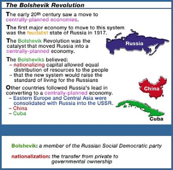
- The Bolshevik Revolution
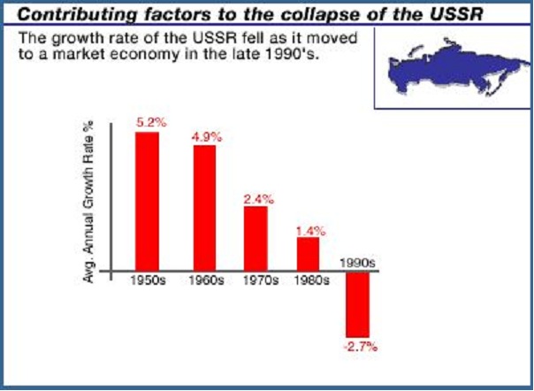
- Contributing factors to the collapse of the Soviet
Union
- Movement back to free-market economy
- The Bolshevik Revolution - the USSR (the Soviet Union) was
formed Dec. 30, 1922
- Forced the movement from a decentralized economy
to a centrally planned economy in Russia in the early
20th century
- they nationalized capital -- the government
took over businesses
- goal was to increase the standard of
living
- With no motivational incentives to produce high
quality goods, production slowed considerably
- in the 1950s and 60s the economy of the Soviet
Union grew at a rate of 5% - 6% -- about the same
or faster than other countries with market
economies
- but in the 1970s this rate slowed to about 2% -
3%, in the 1980s 1% - 2%, and in the 1990s there
was a recession (decline)
- Why?
|
|
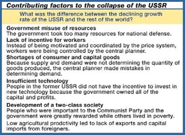
- Contributing factors to the collapse of the Soviet Union
- government took too many resources -- 15% of GDP
used for national defense vs. 6% in the US
- lack of incentives for workers ;ME: the "incentive
problem" from the textbook
- misallocation of resources caused shortages; ME:
the coordination problem from the textbook
- Soviet technology was a decade behind because
there was no profit motive to encourage investment in
new technology
- A two-class society developed
- ME: see the textbook for
- the incentive problem
- the coordination problem
|
|
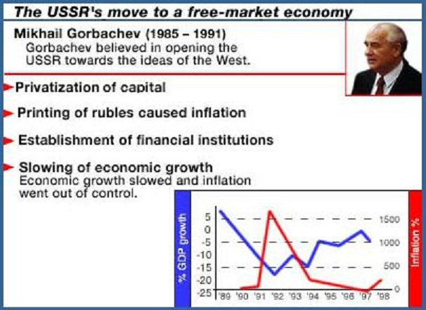
- Movement back to free-market economy
- Mikhail Gorbachev ws the eighth and last leader of
the Soviet Union
- In the late 1980s, through Mikhail Gorbachev's
ideals of glasnost and perestroika, the
Soviet Union began its transformation in response to
the failed planned economy
- Resources were privatized - private ownership
would serve as an incentive to achieve efficiency (ME:
invisible hand)
- Government printed rubles (money) causing
inflation
- prices of goods and services were deregulated and
allowed to be set by supply and demand (ME: chapter
3)
- Problems:
- Russia did not have the financial institutions
that established free market economies did; little
protection of property rights
- organized crime rose in the early 1990s ; a
mafia arose
- Economic growth slowed
|
|
GLOBALIZATION
Why
Venezuela is in crisis
CNN Money 1:49
Optional:
Economic
Systems and Macroeconomics: Crash Course Economics
#3
10:18
- Economic Systems
- Because of scarcity we must
make choices
- what to
produce?
- how to produce?
- who gets it?
- an economic system answers
these three question
- two different economic
system:
- planned or command economy
-
- the government owns the
factors of production (resources)
- government decides how
resources are used
- free market or capitalist
economy
- private ownership of the
factors of production
- laissez-faire
government policies tword the economy, little government
control
- most systems are MIXED
economic systems - some government ownership and some
private
- the invisible hand of
capitalism
- limited resources will go
the most desired use
- ME: allocative
efficiency
- individuals and businesses
meet society's "needs" (ME: I prefer to use the term
"wants") when they seek their own self interest
- ME: it is like there is
an invisible hand guiding their decisions to not only do
what is best for themselves BUT to also do what is best
for society
- ME: the invisible hand
of capitalism achieves efficiency ONLY IF there is
competition
- So do we need a government in
a free market economy? Yes. (ME we'll discuss this more in
lesson 2b)
- to maintain the rule of
law
- public goods and
services
- sometimes competitive
markerts do NOT achieve efficiency and the government needs
to step in like when pollution is created (ME: we will
discuss this in lessons 5a and 5b)
- Modern economies are MIXED
economic systems with both free markets and government
intervention
- Circular Flow Model
- two actors: Households and
businesses
- two markets: product market
and resource market
- but also
government
- Globalization (ME: I sometimes
call this Structural Adjustment)
- Which type of economy is
better and how much should the government get involved?
- very few economists support
command economies and central planning
- trade-offs (opportunity
costs)
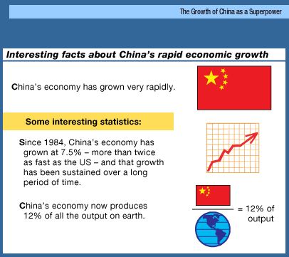
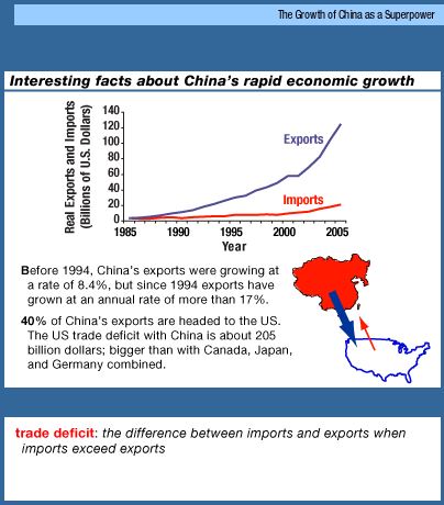
- Chinese leader "Deng
Xiaoping transformed China from a country with debilitating
poverty and famine to economic poserhouse it is today" ME?
How? buy moving away from a centrally planned command
economy toward a free market economy. Result: hundreds of
thousounds of peple were lifted out of poverty!
Optional:
Globalization
and Trade and Poverty: Crash Course Economics
#16
9:01
- 1990s United Nation's Millenium
Goal: by 2015 cut extreme poverty in the world by half
- "extreme poverty = living on
less than $1.25 a day
- Success! But there are still
many very poor people
- Why has extreme poverty
fallen?
- complicated, but
- "greatest contributer (to
the drop in extreme poverty) was globalization and
trade"
- free trade has expanded
greatly
- the poorest one to two billion
people in the world suffer from "globalization deficiency"
which keeps them poor
- benefits of
globalization
- more competition encourages
efficiency
- consumers benefit -- lower
prices
- companies earn more
profit
- low wage foreign workers at
least have jobs
- working conditions are
improving in low wage countries
- downsides
- some jobs displaced
- exploitation and oppression
of poor foreign workers (?)
- different labor rules in
diffent countries
- lack of sustainability and
future environmental problems(?) - ME: when poor people
begin to make more income they consume more resources; poor
people use few resources and richer people use more
resources
- One of the best ways to help the
poor of the world is to help them participate in the economy
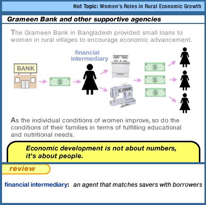
- this includes micro-credit
(ME: Grameen banking)
- "poor people are the world's
greatest entrepreneurs"
Lesson 2b Role of Government and Government
Finance
Role
of Government in a Mixed Economy (YouTube - Daniel Mares)
15:53
- ME: we won't cover "traditional economies"
- The video first reviews the three (four) types of economic
systems that we covered in lesson 2a.
- traditional economy
- command economy
- market economy
- mixed economy
- The five (or six) roles of government in a market economy
- ME our online reading has 5, the video has 6, but the
online reading simply combines two into one.
|
Online Reading
|
Video
|
- Providing the Legal Structure
- Maintaining Competition
- Redistributing Income
- Reallocating Resources
- Correct Externalities
- Provide Public Goods
- Promoting Stability
|
- Maintain Legal and Social Framework
- Maintain Compeetition
- Provide Public Goods and Services
- Redistribute Income
- Stabilize the Economy
- Correct Externalities
|
Where
do your tax dollars go? (YouTube - Test Tube News)
3:44
- 2013 data that does not include Social Security ($800 B) and
Medicare ($500 B)
- ME:
- our textbook (ch.16 on Blackboard) DOES include Social
Security and Medicare
- video only discusses FEDERAL government spending, not state
and local
- video does not discuss from where the tax revenues
come
- Federal Governemnt Spending
- 8% to pay interest on the debt
- 17% on government programs (like agric, administration,
commerce, transportation, research. international affairs,
environment, immigration, education, justice dept. and
others,
- 50% for health care and poverty reduction
("Well-Being")
- 25% on National Defense
When
is a Potato Chip Not Just a Potato Chip (YouTube-LearnLiberty
4:46)
Public
Goods and Asteroid Protection (MRUniversity) 2:30
A
Deeper Look at Public Goods (MRUniversity) 7:55
8.2.2 Analyzing the Tax System (8:19)
OPTIONAL: Tax
Brackets and Progressive Taxation Khan Academy (4:14)
Lesson 3a - Demand
2.1.1 (11:58) Understanding the Determinants of
Demand - 3a
- Outline:
- The determinants of demand
- Building the demand function
- The determinants of demand
- The determinants of demand
- Building the demand function
- The determinants of demand
- ME: In chapter 3 of our textbook the authors list five
"non-price determinants" of demand, but in the video lecture
there are really only 4 non-price determinants of demand. Our
textbook adds: THE NUMBER OF POTENTIAL CONSUMERS that is not in
the video lecture.
- Textbook's non-price determinants of demand: Pe, Pog, I,
Npot, T
- Pe = expected price
- Pog = price of other goods including the price of
complements and the price of substitutes
- I = income
- Npot = the number of potential consumers
- T = tastes and preferences
Video lecture's non-price determinants of demand: Pc, Ps,
M, Ta, Ex
- Pc = price of complementary goods (Pog in the
textbook)
- Ps = price of substitute goods (also Pog in the
textbook)
- M = income (I in the textbook)
- Ta = tastes and preferences (T in the textbook)
- Ex = expected price (Pe in the textbook)
- we will be building a model of the market
- the market is a place where buyers and sellers
trade some good or service determining the price of the
product and the quantity sold; interaction between buyers
and sellers
- demand is the quantity of a good or service that
households want and are able to purchase in a given time
period
- ME: our textbook defines demand as a schedule
that shows the various quantities of a good or
services that consumers are willing and able to buy at
various prices in a given time period, ceteris
paribus
- supply is the quantity of a good or service that
firms want ands are able to sell in a given time period
- ME: our textbook defines supply as a schedule
that shows the various quantities of a good or
services that businesses are willing and able to sell at
various prices in a given time period, ceteris
paribus
- equilibrium is the market condition in which the
interaction of buyers and sellers finds a particular price
and quantity to be traded and from which there is no
incentive to move
- ME: our textbook defines market equilibrium as the
price where the quantity demanded equals the quantity
supplied
- demand describes the behavior of households
- what are the factors (determinants) that influence how much
of a product (bread) consumers will buy?
- the price of bread
- the price of complementary goods (cheese or
bologna)
- the price of substitute goods (bagels)
- income
- tastes and preferences
- expectations of what might happen to the price of bread
in the future
- ceteris paribus assumption: all other factors
are held constant
- the price of bread
- Law of Demand: as the price of a good or service
increases, the quantity purchased generally decreases,
ceteris paribus; there is an inverse relationship
between the price of bread and the quantity demanded
- Why?
- income effect: there is a decrease in
purchasing power when the price of bread
increases
- substitution effect: when the price of
bread increases people will substitute other products
in place of bread and buy less bread
- ME: our textbook adds a third explanation for the
law of demand: diminishing marginal utility --
as we consume more bread we get less extra
satisfaction from each additional piece (i.e. we start
to get sick of it) and therefore we will not buy more
unless the price is lower since we are getting less
satisfaction
- the price of complementary goods (cheese or bologna)
- complementary goods are two goods for which:
- a decrease in the price of one leads to an increase
in the demand for the other, or
- an increase in the price of one leads to a decrease
in demand for the other
- they are goods that are used together like butter or
cheese or bologna that are used along with bread
- so if the price of peanut butter goes up a person will
probably make fewer peanut butter sandwiches and therefor
the demand for bread will go down
- the price of substitute goods (bagels)
- substitute goods are two goods for which
- an increase in the price of one good leads to an
increase in the demand for the other, or
- a decrease in the price of one leads to a decrease in
demand for the other
- so if the price of bagels goes up some people will
switch to bread increasing the demand for bread
- or if the price of bagels falls some people will buy
more bagels instead of bread which will decrease the demand
for bread
- ME: Tomlinson does make a few errors in how he uses the
terms "demand" and "quantity demanded", but he will discuss
and compare these concepts in a later lecture
- income
- normal goods are goods where if your income increases
then the demand for that good will increase
- if you have more money you will buy more normal
goods
- an inferior good is one where if your income increases
demand for the good will decrease
- if you have more money you will buy fewer inferior
goods
- examples: public transportation, potted meat,
beans,
- tastes and preferences
- if people decide that they now like bread better than
they did before then the demand for bread will increase
- ME: the tastes and preferences determinant is often used
for everything else that may influence the demand for a good
or service
- expectations of what might happen to the price of bread in
the future
- if you think that the price will go up in the future
then the demand for bread will go up now
- Building the demand function
- a mathematical expression that shows how the quantity of
bread that household will purchases is a function of these
variables
- Qd = D(Px, Pc, Ps, M, Ta, Ex)
- ME: if we used the determinants and abbreviations from the
textbook then the demand function will look like this: Qd=D(Pe,
Pog, I, Npot, T) or P, P, I, N, T
- NEXT: we will focus our attention on the PRICE of the product
itself and assume that all of the other variables are held
constant, or do not change, this way we will construct the demand
curve
- ME: For MY explanation of the demand and supply determinants
see: http://www.harpercollege.edu/mhealy/eco212i/lectures/ch3-18.htm
2.1.2
(11:54) Understanding the Basics of Demand - 3a
- Outline:
- The demand function
- The demand curve
- The law of demand
- Rationales behind the law of demand
- The demand function
- a mathematical relationship that predicts the quantity of a
good demanded as a function of each of the factors that
influence consumer behavior
- Qd = D(Px, Pc, Ps, M, Ta, Ex)
- ME: if we used the determinants and abbreviations from the
textbook then the demand function will look like this: Qd=D(Pe,
Pog, I, Npot, T) or P, P, I, N, T
- we will focus our attention on the PRICE of the product
itself, ceteris paribus (assuming that all of the other
variables are held constant, or do not change) this way we will
construct the demand curve
- The demand curve
- the graphical relationship between the price of a good and
the quantity demanded, ceteris paribus
- the demand schedule:
- a set of data showing the relationship between price and
quantity demanded, ceteris paribus
- for each possible price of bread there is a quantity
that households will buy in a week, ceteris
paribus
- always label the axes when you draw a graph in economics
- price on the vertical axis and quantity purchased per
week on the horizontal axis
- plot the data from the demand schedule
- note that there are many more prices and many more
quantities that those that we have on our demand schedule so
therefore we can connect the dots on our graph with a smooth
line which is the demand curve
- The law of demand
- the demand curve is downward sloping which shows the law of
demand
- there is an inverse relationship between price and quantity
demanded
- as the price of a good increases, consumers are willing
and able to buy less of it
- as the price of a good decreases, consumers are willing
and able to buy more of it
- note that there are a few exceptions, but in general the
law of demand
- Rationales behind the law of demand -- they explain why the
law of demand is true and why the demand curve is downward sloping
- substitution effect: when the price of bread
increases people will substitute other products in place of
bread and buy less bread
- income effect: there is a decrease in purchasing
power when the price of bread increases
- ME: our textbook adds a third explanation for the law of
demand: diminishing marginal utility -- as we consume
more bread we get less extra satisfaction from each additional
piece (i.e. we start to get sick of it) and therefore we will
not buy more unless the price is lower since we are getting
less satisfaction
2.1.3 (8:13)
Analyzing Shifts in the Demand Curve - 3a
- Shifting the demand curve
- Assuming bread is a normal good, if there is an increase in
household income, what will happen to the demand for bread?
- what will happens to the quantity demanded at each
possible price?
- note: we are keeping the other non-price determinants of
demand constant (ceteris paribus)
- we get a NEW demand schedule so there has been an increase
in demand
- there will be a larger quantity of bread "at every
price"
- on the graph it looks like the demand has shifted to the
LEFT
- ME: note the direction of the arrows. The demand
shifts to the left (horizontally), it does not shift
up and to the right.
- A "Change in Quantity Demanded" vs."Change in Demand"
- this is very important
- they are not the same thing
- a change in quantity demanded is caused by a
change in the price and it is a movement along a single
demand curve
- a change in demand is caused by a change in one of the
non-price determinants of demand (not price) and it results
in a whole new demand curve either to the right
(increase in demand) or to the left (decrease in demand) of
the original demand curve.
- we have a new demand schedule
- we have a new demand curve
- therefore we have a change in demand
- ME: You need to know the difference between a "change in
quantity demanded" and a "change in demand". THEY ARE
NOT THE SAME THING!
- I often ask students in my face-to-face courses "if the
price of pizza increases, what happens to the demand for
pizza?" The correct answer is NOTHING HAPPENS TO THE
DEMAND FOR PIZZA IF THE PRICE OF PIZZA GOES UP.
- If the price of a product changes then there is a
"change in quantity demanded". On the graph you would
move from one point to another point along the SAME DEMAND
CURVE. The demand curve did not change, just the quantity
demanded changed
- In this video lecture we we discussed a "change in
demand" itself, i.e. creating a whole new demand schedule
and demand curve. When there is a change in demand you get a
new demand curve, or the demand curve will shift to to a new
position. This is NOT caused by a change in the price of a
product, but it IS caused by a change in the "non-price
determinants of demand" (Pe, Pog, I, Npot, T) that we held
constant when we developed the demand concept.
2.1.4
(10:43) Changing Other Demand Variables - 3a
- Outline:
- Factors that influence consumer demand
- Variables that shift the demand curve
- Factors that influence consumer demand
- a change in the quantity demanded
- P
 causes Qd
- P
causes Qd
- If the price of a product changes then there is a
"change in quantity demanded"
- the graph does not shift (there has been no change in
demand)
- a change in demand
- a change in one of the non-price determinants of demand
that previously were held constant will cause a change in
demand: a whole new demand curve
- Variables that shift the demand curve
- Video lecture's non-price determinants of demand: Pc, Ps,
M, Ta, Ex
- Pc = price of complementary goods (Pog in the
textbook)
- Ps = price of substitute goods (also Pog in the
textbook)
- M = income (I in the textbook)
- Ta = tastes and preferences (T in the textbook)
- Ex = expected price (Pe in the textbook)
- Textbook's non-price determinants of demand: Pe, Pog, I,
Npot, T
- Pe = expected price
- Pog = price of other goods including the price of
complements and the price of substitutes
- I = income
- Npot = the number of potential consumers
- T = tastes and preferences
- change in the price of other goods -- substitutes
- if there is an increase in the price of bagels, this
will cause an increase in demand for bread (shift to the
right)
- if there is a decrease in price of a substitute good
(bagels), there will be a decrease in demand for the
original product (bread)
- change in the price of other goods -- complementary goods
- if there is an increase in the price of cheese, this
will cause a decrease in demand for bread (shift to the
left)
- if there is a decrease in price of a substitute good
(cheese income), there will be an increase in demand for the
original product (bread)
- change in incomes and normal goods
-
- definition: a normal good is one where demand increase
if income increase
- if incomes increase the demand for normal goods will
increase (shift to the right)
- if incomes decrease the demand for normal goods will
decreases
- change in incomes and inferior goods
- definition: an inferior good is one where demand will
decrease if incomes increase
- Examples: beans, used clothing, potatoes, public
transportation, rice, ramen noodles
- ME: note: a normal good for someone might be a normal
good for someone else
- ME: finally -- "inferior" does not mean "lower quality";
all it means is we will buy less if our incomes increase and
more if our incomes decrease
- if incomes increase the demand for inferior goods will
decrease
- if incomes decrease the demand for inferior goods will
increase
- ME: change in tastes and preferences
- if preferences change in favor of a product then demand
will go up (shift to the right)
- if preferences turn away form a product then demand will
go down (shift to the left)
- change in expected price
- if you expect the price to go up in the future then
demand today will go up (shift to the right)
- if you expect the price to down in the future than
demand today will go down (shift to the left)
- ME: change in the number of potential consumers (see the
textbook)
- if the number of potential consumers increases then
demand for the product will increase (shift to the
right)
- if the number of potential consumers decreases the the
demand for the product will decrease (shift to the
left)
- Summary -- KNOW THIS !!!
2.1.5 (9:16)
Deriving a Market Demand Curve - 3a
- Outline:
- Recall the Demand Function
- The Market Demand Curve
- Recall the Demand Function
- we have been discussing an individual household's demand
for bread
- now we will look at demand for bread in the whole market
where there are many households each with different individual
demand curves
- The Market Demand Curve
- let's assume that there are only two people in the market:
Bob and Ann
- in order to find the market demand we add together the
individual demand schedules; that is at each price we
add the quantities of all the individuals in the market
- graphically the market demand is the horizontal
summation of all individual demand curves in the market
- quantity is on the horizontal axis so when we add the
quantities of all individuals the result is the market demand
is the horizontal summation of all individual demand curves in
the market
- for any price we add the quantity (horizontal distance to
the demand curve) of all people in the market to get the market
demand curve
- anything that shifts the individual demand curves will
shift the market demand curve; the non-price determinants of
demand (Pe, Pog, I, Npot, T) will shift the market demand
curve
Lesson 3b - Supply
2.2.1 (6:00)
Understanding the Determinants of Supply - 3b
- Outline:
- The role of profits
- The determinants of supply
- Factors influencing supply through impact on revenue:
Price
- Factors influencing supply through impact on
costs:Pe, Pres, Pog, Tech, Taxes, Nprod
- The supply function
- The role of profits
- profit = total revenue - total cost
- when profits get larges sellers will be willing to sell
more; when profits get smaller sellers will respond by offering
less for sale
- The Determinants of supply
- Factors influencing supply through impact on revenue:
Price
- total revenue = price x quantity; TR = P x Q
- low prices lead to low revenues, therefore less is
offered for sale by sellers
- high prices lead to high revenues and therefore more is
offered for sale by sellers
- Factors influencing supply through impact on costs: Pe,
Pres, Pog, Tech, Taxes, Nprod
- ME: our textbook discusses six non-price determinants
of supply, the video lecture only discusses four of them
- Pe = expected price
- Pog = price of other goods (textbook only) -- NOTE:
an easier version of this determinant is: price of
other goods also produced by the firm
- Pres = price of resources used to produce the
product
- Technology
- Taxes and Subsidies
- Nprod = number of producers (textbook only)
- Pres = price of resources used to produce the product
- price of the inputs (resources) used to produce the
product (bread)
- if prices of resources are low then costs of
production are low and therefore profits are high AND
businesses will offer more for sale
- if the prices of resources rise AND businesses
will offer less for sale
- Technology
- technology = what you know how to do
- technology = how much output you can get with a given
quantity of inputs
- if technology improves THEN more can be made with the
same number of inputs THEN costs of production are lower
THEN businesses will offer more for sale
- if technology worsens THEN less can be made with the
same number of inputs THEN costs of production are higher
THEN businesses will offer less for sale
- why would technology worsen? it is not likely but
maybe government regulations require a certain, less
productive, technology
- Taxes and Subsidies
- if government taxes businesses it will increase the
costs of production and lose profits, therefore
businesses will offer less for sale
- if the government subsidizes a business, (i.e. gives
it money for producing) then the costs of production will
go down and this will increase profits and businesses
will produce more
- Pe = expected price
- if businesses expect the price of their product
will be higher in the future then they will wait and
produce less today
- if businesses expect the price of their product to go
down in the future they will try to sell more
now
- ME: Pog = price of other goods also produced by the firm
(textbook only)
- if the price of another good also produced by
the same seller goes up, businesses will produce more of
that good and less of the original good
- if the price of another good also produced by
the same seller goes down, businesses will produce less
of that good and more of the original good
- ME: Nprod = number of producers (textbook only)
- if the number of sellers (or producers)
increases then businesses will be able and willing to
produce more
- if the number of producers goes down, then businesses
will produce less
- The supply function
- the quantity of a product that businesses are willing to
sell will depend on: the price, price of resources, technology,
taxes and subsidies, expected price, price of other goods, and
the number of producers
- the supply function is a mathematical relationship that
predicts the quantity of a good supplied as a function of each
of the factors that influence supplier behavior
- Qs = S(P, Pr, T, G, Ex Pog, Nprod)
- ME: Qs = S(P, Pe, Pog, Pres, Tech, Tax, Nprod)
2.2.2 (9:49)
Deriving a Supply Curve - 3b
- Outline:
- The supply function
- The supply curve
- The law of supply
- Rationale behind the law of supply
- The supply function
- Qs = S(P, Pi, T, G, Ex Pog, Nprod)
- ME: Qs = S(P, Pe, Pog, Pres, Tech, Tax, Nprod)
- in this video lecture will look at the relationship between
the price of a good and the quantity supplied HOLDING CONSTANT
all of the other factors (determinants); how does the price of
a product affect the quantity supplied, ceteris
paribus?
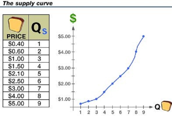
- The supply curve
- the supply schedule is a set of data
(table) showing the relationship between price and the
quantity supplied, ceteris paribus;
- low prices lead to low revenues, therefore less is
offered for sale by sellers
- high prices lead to high revenues and therefore
more is offered for sale by sellers
- convert the supply schedule into a supply graph
- always label the axes
- quantity on horizontal axis and price on the
vertical axis
- plot the data and connect the dots
- ME: the study guide has problems where YOU
can do the actual graphing; if graphs confuse or
worry you then you should do these
problems
- the supply curve shows the graphical
relationship between the price of a good and the
quantity supplied, ceteris paribus
|
|
- The law of supply
- supply curves slope upward this indicates a direct
relationship between price and quantity supplied
- the law of supply states that as the price of a good
or service increases, the quantity offered for sale generally
increases
- Rationale behind the law of supply
- ME: we will always explain the shape of the graphs that we
draw; we have already done this with the production
possibilities curve and with the demand curve; make sure you
understand the shapes of all the graphs in this
course.
- the law of increasing opportunity costs helps
explain the law of supply
- opportunity cost is the best alternative that is
given up; when a choice is made
- the more bread that a baker offers for sale, the higher
the cost of producing each additional loaf
- Why?
- the supply curves slopes upwards because the opportunity
costs rise as the business produces more and more, so they will
need a higher price or they will decide to do something
else
- also, we will see in a later video lecture that the supply
curve slopes upwards because the marginal costs (the extra
costs of producing one more, increase
- ME: the textbook offers these explanations for the law of
supply:
- higher prices mean higher revenue for the producer which
is an incentive for he producer to produce more
- as quantity increases the added cost of producing one
more unit of output (called the marginal cost) increases
because the factory will start to get crowded
- finally, I like to add the law of increasing cost that
we used to explain the shape of he production possibilities
curve, since all resources are not eh same as we increase
production of a good we will have to use less suitable
resources (like less qualified workers) which ill increase
coses. so, businesses will not produce more at a higher cost
unless they can get a higher price to cover those higher
costs
2.2.3 (6:52)
Understanding a change in Supply versus a Change in Quantity Supplied
- 3b
- Outline:
- Reviewing supply
- Supply and changes in the input prices
- Graphing a change in supply
- Change in quantity supplied vs. change in
supply
- Reviewing supply
- when we drew the supply curve we saw how the quantity
produced changed as we changed the price, ceteris
paribus
- ceteris paribus means that we held constant
everything else; only the price and quantity changed
- determinants that were held constant"
- Pi, T, G, Ex
- ME: Pe, Pog, Pres, Tech, Tax, Nprod
- but what happens if these other factors (ME: our textbook
calls these the "non-price determinants of supply")
change?
- in this lessen we will only look at a change in input
(resource) prices, then int he next video lecture will will
look at the other factors (determinants) of supply
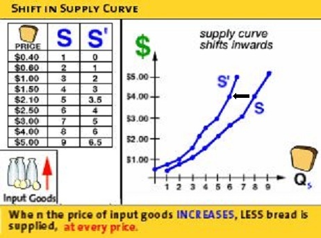
- Supply and changes in the input prices (price of
resources)
- what happens if the price of resources used to
produce the good (inputs) increase?
- profit will go down
- and businesses will produce less
- on the supply schedule we will see a smaller
quantity supplied AT EVERY PRICE;
- so on the supply schedule we will see lower
quantities supplied; at each price the quantity
supplied is lower; there is a new supply
schedule
- Graphing a change in supply
- so if the price of inputs goes up, this will cause
the supply curve to shift (move) to the left
- so on the supply curve there is a new supply
curve further to the the left; the supply has
DECREASES (shifted to the left)
|
|
- Change in quantity supplied vs. change in supply
- A change in the price of bread will cause a change in
quantity supplied which is a movement along a single supply
curve
- if one of the non-price determinants of supply change then
we get a whole new supply curve and we call this a change in
supply
- an increase in supply means the supply curve
shifts to the left
- a decrease in supply means the supply curve
shifts to the right
2.2.4 (8:47)
Analyzing Changes in Other Supply Variables - 3b
- Outline:
- Factors that influence producer's behavior
- Changes in the price of the product
- Changes in variables held constant when drawing the
supply curve
- VIDEO: Pi, T, G, Ex
- ME: Pe (Ex), Pog, Pres (Pi), Tech (T), Taxes (G),
Nprod
- Factors that influence producer's behavior
- VIDEO: Qs = S(P, Pi, T, G, Ex )
- ME: Qs = S(P, Pe, Pog, Pres, Tech, Tax, Nprod)
- Changes in the price of the product
- if the price of changes then there is a movement ALONG the
supply curve because price is already on the vertical axis
- we call this a change in the quantity supplied
- Changes in variables held constant when drawing the supply
curve
- VIDEO: Pi, T, G, Ex
- ME: Pe (Ex), Pog, Pres (Pi), Tech (T), Taxes (G),
Nprod
- if there is a change in one of these variables them the
supply schedule changes and we get a whole new supply
curve
- we call this a change in supply
- Pi
(change in the price of resources or inputs; Pres)
- if the price of resources increases then costs
increase and supply decreases -- shifts to the
left
- if the price of resources decreases then costs
decrease and supply increases -- shifts to the
right
- NOTE: a shifting of the demand curve means the the
quantity changes AT EACH POSSIBLE PRICE
- an increase in supply means the quantity
supplied increases at each possible price and the supply
curves shifts to the right
- a decrease in supply means that the quantity
supplied at each possible price decreases and the supply
curve shifts to the left
("
"means "change in")
- T
(change in technology)
- if the technology improves then productivity
increases and costs of producing the product will decrease
and supply increases -- shifts to the right
- if the technology gets worse then productivity
decreases and costs of producing the product will increase
and supply decreases -- shifts to the left
- G
(changes in taxes and subsidies)
- if taxes increase then costs of production
increase and supply decreases -- shifts to the
left
- if taxes decreases then costs of production
decrease and supply increases -- shifts to the
right
- if subsidies increase then costs of production
decrease and supply increases -- shifts to the
right
- if subsidies decrease then costs of production
increase and supply decreases -- shifts to the
left
- Ex
(change in expected price; Pe)
- if sellers expect the price to increase in the
future then supply today will decrease -- shift to
the left
- if sellers expect the price to decrease in the
future then supply today will increase -- shift to
the right
- ME: Pog
(change in the price of other goods also produced by the firm)
- if a producer produces to different products, let's say
corn and soybeans, then if the price of corn
increases then producers will produce more corn and
the supply of soybeans will decrease -- shift to the
left; why plant soybeans if they can get a higher price for
their corn?
- if a producer produces to different products, let's say
corn and soybeans, then if the price of corn
decreases then producers will produce less corn and
the supply of soybeans will increase -- shift to the
right; they will be willing to sell more soybeans at each
possible price since profits from corn are lower
- ME: Nprod
(change in the number of producers)
- if the number of producers increases then supply
increases -- shifts to the right
- if the number of producers decreases then supply
decreases -- shifts to the left
2.2.5 (7:16)
Deriving a Market Supply Curve from Individual Supply Curves -
3b
- Outline:
- Recall the supply function
- The market supply curve
- Recall the supply function
- VIDEO: Qs = S(P, Pi, T, G, Ex )
- ME: Qs = S(P, Pe, Pog, Pres, Tech, Tax, Nprod)
- The market supply curve
- market supply is the horizontal summation of all of
the individual supply curves in the market
- for the market supply schedule we add up the
quantities at each price for ALL PRODUCERS; prices stay the
same and the quantities are added together
- therefore the market supply curve will be further to
the right as we add more producers
- since the quantity is on the horizontal axis we call this
horizontal summation; prices stay the same and the
quantities are added together
- What will shift the market supply curve?
- answer: anything that shifts the individual supply
curves
- VIDEO: Pi, T, G, Ex
- ME: Qs = Pe, Pog, Pres, Tech, Tax, Nprod
- ME:
- REMEMBER: a change in the price of the product itself
will NOT shift (change) the supply curve
- if the price of corn increases what will happen to the
supply of corn? Answer: NOTHING
Lesson 3c - Market Equilibrium and Efficiency
- PUTTING SUPPLY AND DEMAND TOGETHER
- MARKETS AND EFFICIENCY
2.3.1
(11:04) Determining a Competitive Equilibrium - 3c
- Outline:
- Definition of competitive equilibrium
- Excess demand
- The bidding mechanism
- Excess supply
- A competitive equilibrium
- Definition of competitive equilibrium
- we will be putting what we have learned about demand and
supply together to create a model that will help us to predict
how factors in the environment will affect the price of a
product
- why are prices what they are and what makes price
change?
- competitive equilibrium:
- assumptions:
- there are many buyers and sellers in the market
- who have no influence over the price; i.e. they are
price takers
- competitive equilibrium occurs at the price where
the quantity supplied equals the quantity demanded
- equilibrium means that we have a situation in
which there is no tendency to change; a situation in which
neither consumers or firms have any incentive to change
their behavior
- there will be only one price in which there is no
pressure for something to change and that is the price where
the quantity demanded (Qd) equals the quantity supplied
(Qs); Qd=Qs
- graphically: the equilibrium will be the price where the
demand and supply curve cross; this is the price where
Qd=Qs
- Excess demand
- if the price is below the equilibrium then the Qd
> Qs and there will be excess demand
- Excess demand is the difference between the Qd and
the Qs when consumers demand a greater quantity than the
suppliers are willing and able to supply; i.e. when the price
is below the equilibrium price
- if there is excess demand then there will be a
shortage
- The bidding mechanism
- if the price is below the equilibrium then the
excess demand this will cause the price to go up so this is not
the equilibrium
- this is called the "bidding mechanism"; this is the
process by which unsatisfied buyers try to change the price of
a good in order to guarantee that they are able to obtain it;
unsatisfied buyers will be willing to pay a higher price to get
the product
- Tomlinson uses the term "reservation price"
- the bidding mechanism will continue to drive the price up
until the Qs=Qd and there is no more excess demand
- Excess supply
- if the price is above the equilibrium price then the Qd
< Qs and there will be excess supply, or a
surplus
- excess supply (or a surplus) is the difference between the
quantity supplied and quantity demanded when producers supply a
greater quantity than consumers are willing to buy; i.e. if the
price is too high
- if there is an excess supply the bidding mechanism will
cause the price to fall as sellers try to sell off their
surplus
- as the price goes down the quantity demanded will increase
and the quantity supplied will decrease; this means we will
move down along the demand and supply curves until we reach the
price where Qd = Qs or where the curves cross
- A competitive equilibrium
- occurs at the price where the quantity demanded by buyers
and the quantity supplied by producers are equal
- now there is no excess demand and no excess supply; there
is no further tendency to change; equilibrium has been
reached
- on the graph the equilibrium will occur where the supply
curve and the demand curve intersect (cross)
2.3.2 (7:02)
Defining Comparative Statics - 3c
- Outline:
- Competitive Equilibrium
- Three steps to finding a new equilibrium when a
non-price determinant changes
- identify which side of the market is affected? (will
it change demand or supply?)
- how does the change affect the curve? (will demand or
supply increase [shift right] or decrease [shift
left]?)
- how does the equilibrium change? (use the graph to
see what happened to the equilibrium price and
quantity)
- ME: Our textbook does not use the term "comparative statics",
but instead uses the term "equilibrium" which is also used in the
video lectures
- Competitive Equilibrium
- equilibrium occurs at the price where the Qs = Qd
- equilibrium will be at the price and quantity where the
supply and demand curves cross
- Three steps to finding a new equilibrium when a non-price
determinant changes
- we can use our model (graph) to predict, or explain, how
something in the environment (real world) affects the
equilibrium price and quantity of a product
- anytime that there is a change in one of the non-price
determinants of demand or supply then there will be a change
int he equilibrium price and quantity
- Tomlinson says that there are three steps:
- identify which side of the market is affected? (will it
change demand or supply?)
- how does the change affect the curve? (will demand or
supply increase [shift right] or decrease [shift
left]?)
- how does the equilibrium change? (use the graph to see
what happened to the equilibrium price and quantity)
- ME: Four steps
- first determine which non-price determinant has changed
- there are five non-price determinants of demand: Pe,
Pog, I, Npot, T (P, P, I, N, T)
- there are six non-price determinants of supply: Pe,
Pog, Pres, Tech, Tax, Nprod (P, P, P, T, T, N)
- if one of these 11 determinants change then we will
get a change in the price and quantity of the
product
- identify which side of the market is affected? (will it
change demand or supply?;
- did a non-price determinant of demand change? or
- did a non price determinant of supply change?
- will demand or supply increase [shift right] or
decrease [shift left]?
- how does the equilibrium change?
- GRAPH IT!
- then use the graph to see what happened to the
equilibrium price and quantity)
- do not try to guess; draw the graphs and shift
a curve and then you can see what happens to the
equilibrium price and quantity
- example:
- what would happen to the price of bread and the quantity
sold if the price of bagels, a substitute good, increases;
price of bagels goes up so what happens to the market for
bread?
- 4 steps:
- first determine which non-price determinant has changed
- demand: Pe, Pog, I, Npot, T
- supply: Pe, Pog, Pres, Tech, Tax, Nprod
- the non-price determinant that has changed is: POG -
substitute
- will it change demand or supply?
- since price of substitutes is a determinant of
demand, then the demand curve will shift
- how does the change affect the curve?
- we have learned that if the Pog-sub goes up
this will increase demand for our product
- price of bagels increasing will cause the demand
for bread to increase
- how does the equilibrium change?
- GRAPH IT!
- shift the demand to the right
- at the original price and with the new demand curve
we can see that there will now be excess demand
(Qd>Qs); this will create and excess demand and the
bidding mechanism will bid the price up
- from the graph we can see that if the price of
bagels increases this will cause the price
of bread to increase AND people will buy more
bread
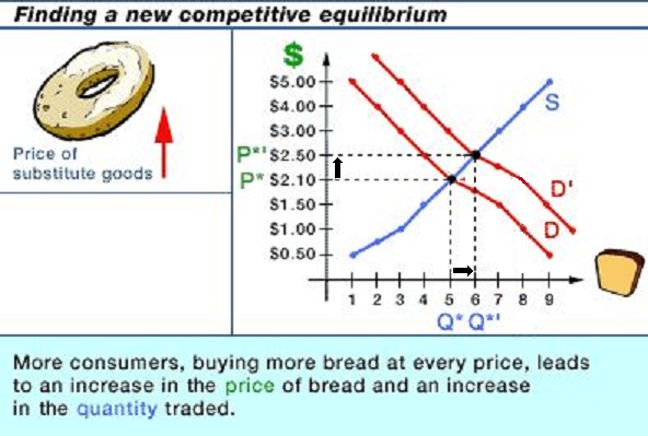
2.3.3 (13:04) Classifying Comparative Statics
(should be 3.4-2, but the link works) - 3c
- Outline:
- Comparative statics
- The demand curve shifts outward (increase in
demand)
- The demand curve shifts inwards (decrease in
demand)
- The supply curve shifts outwards (increase in
supply)
- The supply curve shifts inwards (decrease in
supply)
- ME: Our textbook does not use the term "comparative statics",
but it does discuss how the non-price determinants of demand and
supply affect the equilibrium price and quantity and that is what
the video lecture does here
- Comparative statics
- comparative statics is comparing one state (condition) of a
competitive equilibrium to another when one of the variables
affecting demand or supply changes
- ME: NOTE --
- Goal: to see what happens to the price of a good and the
quantity traded (sold) when we change one of the variables
that we usually hold constant when drawing the supply and
demand curves
- there are only four possibilities:
- The demand curve shifts outward (increase in
demand)
- The demand curve shifts inwards (decrease in
demand)
- The supply curve shifts outwards (increase in
supply)
- The supply curve shifts inwards (decrease in
supply)
- ME: but more than one variable could change at the same
time including one or more of demand and one or more of supply;
our textbook has example of these
- The demand curve shifts outward (increase in demand)
- demand shifts to the right causing the price to increase
and the quantity to increase
- results in a shortage of the good at the original
price
- the price and quantity sold will increase
- what could cause an increase in demand?
- The correct change in the textbook's non-price
determinants of demand:
- Pe = expected price
- Pog = price of other goods including the price of
complements and the price of substitutes
- I = income
- Npot = the number of potential consumers
- T = tastes and preferences
- KNOW THESE!!
- The demand curve shifts inwards (decrease in demand)
- demand shifts to the left causing the price to decrease
and the quantity to decrease
- What would cause a decrease in demand?
- The supply curve shifts outwards (increase in supply)
- supply shifts to the right causing the price to decrease
and the quantity to increase
- This would cause a surplus and the price will begin to
drop
- What would cause an increase in supply?
- The correct change in the textbooks non-price determinants
of supply
- a change in the expected price (Pe,)
- a change in the price of another good also produced by
the firm (Pog)
- a change in the price of resources (Pres)
- a change in technology (Tech,)
- a change in taxes or subsidies
- a change in the number of producers (Nprod)
- KNOW THESE!
- The supply curve shifts inwards (decrease in supply)
- supply shifts to the left causing the price to increase
and the quantity to decrease
- What would cause a decrease in supply?
- KNOW THESE!
3c - MARKETS AND EFFICIENCY
Supply, Demand, and Economic
Efficiency - 3c
Read: http://www.harpercollege.edu/mhealy/eco211/lectures/s%26d/sdeff.htm
EC
Efficiency and Equilibrium in Competitive Markets (11:48) - 3c
Free at: http://www.econclassroom.com/?p=2611
uses benefit cost analysis
- Efficiency exists in a society when no individual in
society can be made better off without making someone else worse
off
- Allocative efficiency occurs when the MB = MC (MSB = MSC)
- the demand curve is downward sloping indicating that society
is getting less extra satisfaction (MB) from consuming more
- the supply curve is upward sloping since the MC of producing
more goes up as resources become more scarce (ME: AND as we need
to use less suited resources to produce our product)
- Allocative efficiency occurs at the equilibrium price and
quantity because the total of consumer and producer surplus is
maximized at the equilibrium; ME: this is also where the MB = MC
(MSB = MSC)
- what if the quantity is less than the equilibrium quantity?
- we get allocative inefficiency because the MSB >
MSC
- we say that we have an underallocation of resources;
too few resources are being used to produce the product; we are
getting a lot of benefits (MB is high) and the costs to
society is low (MC is low)
- this means we want more or we would be happier if we had
more
- there is also a loss of total surplus to society; even
though producer surplus may increase, consumer surplus
decreases a lot and there is a loss to society, called the
dead weight loss (or welfare loss; "welfare" means
satisfaction)
- society is less satisfied and we have allocative
inefficiency
- what if the quantity was greater than the equilibrium
quantity?
- we get allocative inefficiency because the MSB <
MSC
- we say that we have an overallocation of resources;
too many resources are being used to produce the product; we
are getting few benefits (MB is low) and the costs to
society is high (MC is high)
- this means we want more or we would be happier if we had
less of this product (and more of something else that makes us
happier)
- in order to get producers to produce more they would need a
higher price
- this would decrease consumer surplus and even though
producer surplus would go up a little th3ere is a net loss to
society, the dead weight loss
- in a market economy society's satisfaction is maximized at the
equilibrium price and quantity
- ME:
- of course the equilibrium price ans quantity is WHAT WE
GET, because it is here that producers will make the biggest
profit
- the allocatively efficiency quantity is WHAT SOCIETY WANTS
because they maximize their satisfaction
- in a competitive market economy (with no externalities --
chapter 5) WHAT WE GET = WHAT WE WANT and we achieve allocative
efficiency
- This is the "invisible hand" of capitalism that
Friedman discussed in the previous video in chapter 2
[Power
of the Market (YouTube LibertyPen 1:14)]
Lesson 20a -Why we Trade: Comparative
Advantage
SPECIALIZATION AND GAINS FROM TRADE
1.5.1 (22:40) Defining Comparative Advantage
with the Production Possibilities Curve - 2a
- Outline
- Anne's Production Possibilities
- Comparing Production Possibilities curves
- Specializing and Trading
- Creating More Output
- Anne's Production Possibilities
- ME:
- The concept of comparative advantage can be used to show
how two (or two countries) with different abilities (or
resources) can cooperate (or trade) to increase their
wealth
- we will show how countries gain from international
trade
- we will be using straight line production possibilities
curves for two different people (Bernie [previous
lecture] and Anne) to show how together they can do more
than if they cooperate (trade)
- Note that Anne can BOTH scrub and sweep more than can
Bernie; we say that Anne has an absolute advantage in
doing both tasks since she can do them with fewer resources;
i.e. Anne is better at doing both
- Anne's production possibilities schedule shows the various
maximum combinations of sweeping and scrubbing maximum number
of rooms that she can do in one hour
- Comparing Production Possibilities curves: finding the
opportunity costs
- Calculate Anne's opportunity costs of sweeping and
scrubbing"
- 1 room swept = 1 room not scrubbed
- 1 room scrubbed = 1 room not swept
- Calculate Bernie's opportunity costs
- 1 room swept = 1/2 room not scrubbed
- 1 room scrubbed = 2 room not swept
- a straight line PPC means that the opportunity costs are
constant; for a country it would mean that we would assume a
that all resources within that country are the same; remember
in a previous lecture we said that a PPC is usually concave to
the origin (bowed out) because not all resources are the
same. Some are better for producing one product and others are
better suited to producing something else
- this causes the opportunity costs to increase as we
produce more of one product
- i.e. this causes the shape of the PPC to be concave
(bowed out)
- BUT when discussing comparative advantage we usually assume
that all resources within a country are the same so that we get
constant opportunity costs and a straight line PPC: this makes
our work easier
- Specializing and Trading
- Here are the opportunity costs again:
- Anne's opportunity costs of sweeping and
scrubbing
- 1 room swept = 1 room not scrubbed
- 1 room scrubbed = 1 room not swept
- Bernie's opportunity costs
- 1 room swept = 1/2 room not scrubbed
- 1 room scrubbed = 2 room not swept
- What if they worked independently:
- then they can only sweep and scrub a number of rooms
that is on their PPC
- lets ASSUME that Bernie sweeps 2 rooms and scrubs 2
rooms
- lets ASSUME that Anne sweeps 6 rooms and scrubs 6
rooms
- they of course could clean different combinations, but
let's just use this as our given starting point
- Creating More Output
- working independently, what are the total number of rooms
that are swept and scrubbed?
- scrubbing: Bernie 2 rooms + Anne 6 rooms = 8 rooms
scrubbed
- sweeping: Bernie 2 rooms + Anne 6 rooms = 8 rooms
swept
- remember this is one of the MAXIMUM combinations
possible if they work independently
- But what if they specialize according to their
comparative advantages? Then, how many rooms can be scrubbed
and swept?
- a person has a comparative advantage at an activity
if they can perform that activity at a lower opportunity cost
than anyone else; i.e. if they give up less than other
people when they do the activity
- We will show that if Bernie and Anne specialize according
to their comparative advantages that they can scrub and sweep
MORE ROOMS THAN IF THEY WORKED INDEPENDENTLY
- who has a comparative advantage in scrubbing? --
that is, who has a lower op cost of scrubbing OR who gives
up sweeping fewer rooms when they scrub
- ANNE: 1 room scrubbed = 1 room not swept
- Bernie: 1 room scrubbed = 2 room not swept
- Anne has a lower op cost of scrubbing = 1room
not swept; if she scrubs a room she gives up fewer rooms
not swept -- just 1) whereas If Bernie scrubbed a room he
would give up 2 rooms not swept.
- so Anne has a comparative advantage in
scrubbing and she should specialize in scrubbing
- who has a comparative advantage in sweeping? --
that is who has a lower op cost of sweeping OR who gives up
scrubbing fewer rooms when they sweep
- ANNE: 1 room swept = 1 room not scrubbed
- Bernie: 1 room swept = 1/2 room not scrubbed
- Bernie has a lower op cost of sweeping = 1/2 room not
scrubbed; if he sweeps a room he gives up fewer rooms not
scrubbed -- just 1/2) whereas If Anne swept a room she
would give up 1 rooms not scrubbed.
- so Bernie has a comparative advantage in sweeping
and he should specialize in sweeping
- People, or countries, should specialize in (do more of)
those things in which they have a comparative advantage; in
which they give up the least. When they do this MORE will
be produced
- We will see how in the next lecture
1.5.2
(6:46) Understanding Why Specialization Increases Total Output -
2a
- Outline
- Bernie and Anne Continued
- Recognizing specialization
- Conclusion
- Bernie and Anne Continued
- Bernie has a comparative advantage in sweeping and he
should specialize in sweeping
- Anne has a comparative advantage in scrubbing and she
should specialize in scrubbing
- So lets have Bernie ONLY SWEEPS and in one hour he will be
able to sweep 6 rooms (and scrubbing 0)
- And, let's have Anne do more scrubbing, let's say she
scrubs 9 rooms. leaving her time to sweep 3 rooms
- What happened to total number of rooms scrubbed and swept?
- by specializing according to their comparative
advantages together they are now sweeping 9 rooms (6 by
Bernie and 3 by Anne) and scrubbing 9 rooms (all by
Anne)
- REMEMBER: in the previous lecture we said that working
independently they could only sweep and scrub 8 rooms, BUT by
specializing and trading they can now sweep and scrub 9 rooms,
in the same amount of time
- BEFORE (without specialization):
- scrubbing: Bernie 2 rooms + Anne 6 rooms = 8 rooms
scrubbed
- sweeping: Bernie 2 rooms + Anne 6 rooms = 8 rooms
swept
- AFTER (with specialization):
- scrubbing: Bernie 0 rooms + Anne 9 rooms = 9 rooms
scrubbed
- sweeping: Bernie 6 rooms + Anne 3 rooms = 9 rooms
swept
- ME: with the same amount of resources (one hour of work
each), by specializing according to their comparative
advantages, MORE ROOMS were swept and scrubbed (one more of
each)! EVEN THOUGH Anne is better at doing both.
- Recognizing specialization
- Conclusion
- the trader with the flatter PPC will have a comparative
advantage for providing the good or service on the horizontal
axis (assuming the graphs are calibrated the same)
- if you have a comparative advantage in one good then you
have a comparative disadvantage for the other good
- everyone has a comparative advantage in something
- by specializing according to comparative advantage
everyone who is trading can gain!
1.5.3 (25:35) Analyzing International Trade
Using Comparative Advantage - 2a
- Outline
- Constraints of Two Countries
- Graphing Production Possibilities
- Benefits of Trading
- Constraints of Two Countries
- Pakistan's unit labor requirement: the amount of time it
takes to perform a task
- 1 wheat takes 2 workers
- 1 rice takes 3 workers
- now we can calculate the opportunity cost
- 1W = 2/3 R
- 1R = 3/2 W = 1 1/2 W
- if Pakistan has only 60 workers then it can produce
- a maximum of 30 W
- OR a maximum of 20 R
- now we can draw the PPC for Pakistan
- Malaysia with a different technology can produce
- 1 W with 1 worker, and
- 1 R with 2 workers
- Malaysia has an absolute advantage in producing both
wheat and rice; i.e. they are better at producing both
- now we can calculate the opportunity costs in Malaysia
- 1 W= 1/2 R; every time they produce a bushel of wheat
it takes them 1 worker who could have produced 1/2 bushel
of rice
- 1 R = 2 W
- if Malaysia has only 60 workers then it can produce
- a maximum of 60 W
- OR a maximum of 30 R
- now we can draw the PPC for Malaysia
- Graphing Production Possibilities
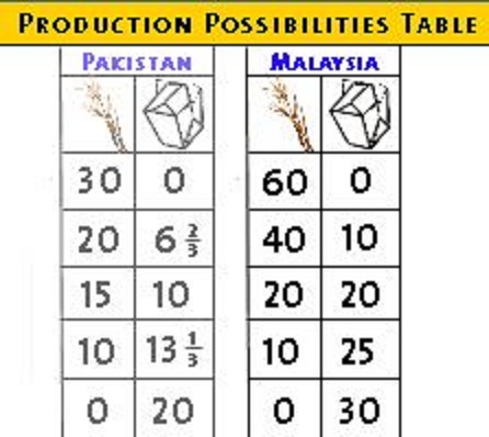
- PPC is a straight line
- which means the opportunity cost is constant; it means we
are assuming all of the resources in Pakistan are the same and
all of the resources in Malaysia are the same;
- if some resources in one country were better at producing
wheat and some were better at producing rice then the PPC would
be concave (bowed out) and we would have increasing costs
- we could have also plotted the PPC using the equation for a
straight line
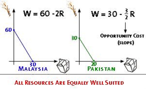
- opportunity costs again and now we can see which country has a
comparative advantage in which product:
- Benefits of Trading: Showing how both countries can gain from
specialization and trade
- you will be given an initial starting point when countries
are not trading; when they are independent of each
other; one of the points along their PPC
- BEFORE (this will be given to you):
- Malaysia: 20 R and 20 W
- Pakistan: 10 R and 15 W
- total production when acting independently: 30 R and
35 W
- how can they gain if they specialize according to their
comparative advantage and trade?
- opportunity costs again and now we can see which country
has a comparative advantage in which product:
- find comparative advantage:
- Pakistan because its op cost of rice (3/2) is lower
than the op cost of rice in Malaysia (2 W); so Pakistan
has a comparative advantage in rice and it should produce
more rice
- Malaysia has a comparative advantage in wheat (2/3 is
less than 2); so Malaysia should produce more wheat
- AFTER - Gains from trade:
- IF Pakistan produces ONLY RICE it can produce
20R
- if Malaysia produces 12 R it can still produce 36
W
- totals with trade: 32R and 36 W
- total (from above) without trade: 30 R and 35
W
- GAINS from trade: 2 more R and 1 more W have been
produced with the same amount of
resources
- ME: our textbook discusses 100% specialization
meaning the Pakistan only produces rice and Malaysia only
produces wheat. Lets see how both countrys can gain from trade:
- assume BEFORE they specialize:
- Pakistan produces15W and 10 R, and
- Malaysia produces: 40 W and 10 R
- Total BEFORE specialization: 55W and 20 R
- now if both countries only produce the products in which
they have a comparative advantage (100% specialization)
- Pakistan produces 20R, and
- Malaysia produces: 60W
- Total AFTER specialization: 60W and 20 R
- Gains from specialization and trade (compare BEFORE
with AFTER): 5 more W are bing produced from the same
amount of resources if the countries trade.
1.5.4 Outsourcing
8:54
- Up to 3.3 million white jobws will move to other countries
like india in the next 10 years (2004 - 2014). Should we be
concerned?
- Outsourcing:
- Definition: the practice whereby a firm gets sevices
previously provided by its own workers by a new third party
provider outside the firm. Contracting with an outside
provider.
- Net effect on the economy:
- effect on employment is insignificant -- less workers at
the original firm but more workers at the outside
provider,
- BUT since the new outside provider is a specialist they
will probably be able to provide tje service at a lower
cost
- Off-shoring:
- Definition: the practice whereby a firm gets sevices
previously provided in this country from
resources located in another country. Outsourcing to another
country
- Net effect on the economy
- off-shoring leads to some loss of jobs
- foreign workers have a higher standard of living and
they may buy some imports produced in the original country
which would increase employment but probably at a lower wage
or with retraining costs
- Benefits of off-shoring far exceed the costs
- Bernefitt: large cost savings for companies in this
country that off-shore services and this can lead to
lower prices
- Benefits of 24 hour a day operations with service
centers scattered around the world and enhanced
productivity
- Benefits: additional income and jobs due to extra
exports
- Costs: unemployment or lower wages
- Is it fair?: Off-shoring is similar to technological
advancement that replaces labor. Who complains that new
computer technology has cost some jobs?
- Limits of off-shoring
- automation is moving some jobs back to the US
- higher wages in other countrys is sometimes making it
more profitable to bring the jobs back
- So what should you do to avoid losing your job to
off-shoring
- education!
- many more jobs are created than are destroyed
- technological progress and integration of the world
economy are big opportunities
17.4.3 Hot
Topic: Winners and Losers in NAFTA 4:20
- NAFTA = North American Free Trade Agreement = freer trade
between the US, Canada, and Mexico
- economic integration is changes in goavernment policy and
trade liberalization that make international commerce easy
- ME: part of strudtural adjustment = joining the world
economy
- trade liberalization: reducing trade barriers like tariffs
(txes on imported products) and quotas (limits on the quantity of
a good that can be imported
- NAFTA went into effect in January 1994 beginning a fifteen
year phasing out of tariffs and quotas
- Effects of NAFTA 1994-2004
- trade between the US and Mexico increased 70%
- many new jobs have been created
- factories have been built along the US-Mexican border to
take advantage of this new trade
- more economic growth
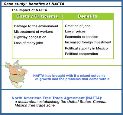
Lesson 20b - International Trade and Exchange
Rates
17.1.1 Determining
the Difference between a Closed Economy and an Open
Econonmy 8:55
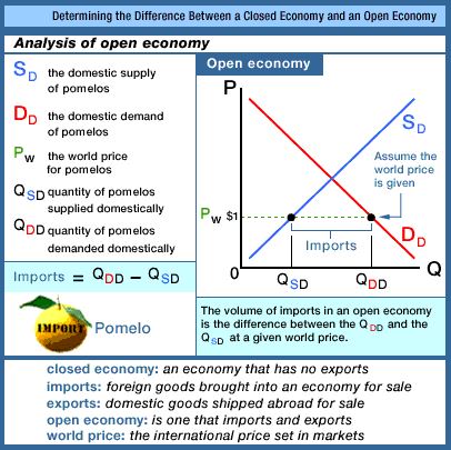
17.4.2 Trade
Policy 7:17
- The Effect of Government Policy on International Trade
- Definitions
- an closed economy is an economy that does not trade
internationally
- an open economy is an econmy that trades
internationally
- a tariff is a tax imposed on internationally traded
goods
- a quota is a restriction on the quantity that one country
can import from another
- Effects of a tariff:
- higher prices
- less consumption
- less imports and more domestic production
- increasing value of domestic currency (the dollar
appreciates)
|
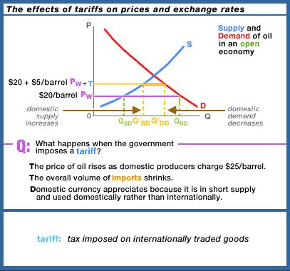
|
- Effects of a Quota
- higher prices
- less consumption
- less imports and more domestic production
- increasing value of domestic currency (the dollar
appreciates)
|
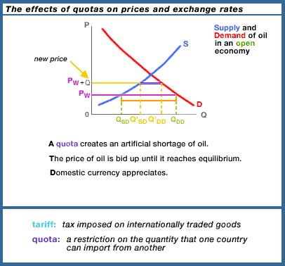
|
MJM 35 Why
do Countries Restrict Trade? (8:34)
MJM 36 Types
of Trade Restrictions (9:43)
- ME: Here are the trade nrestrictions discussed in the
textbook:
- a. tariffs
1) revenue tariffs
2) protective tariffs
b. import quotas
c. nontariff barriers
d. voluntary export restrictions
e. export subsidies ( a barrier to trade?)
|
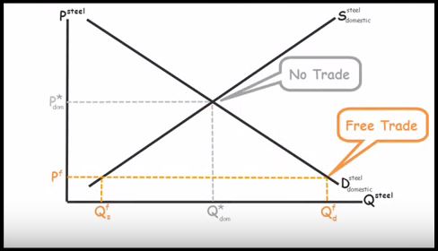
|
- Tariff: a tax on imported goods
- Effects: who wins with a tariff
- the domestic industry
- domestic workers
- government gets tariff revenue
- Effects: who loses:
- domestic consumers have higher prices
- domestic consumers have a smaller quantity than
under free trade
- the foreign producer and their workers
|
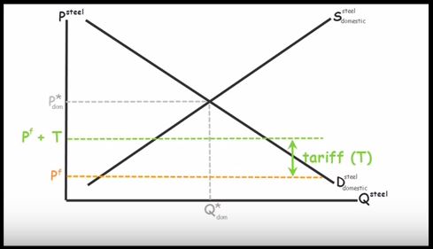
|
- Quota: a limit on the quantity or value that can be
imported
- Effects: who wins?
- domestic producers
- domestic workers
- Effect: who loses?
- domestic consumer
- foreign producers
- ME: though the video says that tariffs and quotas
have the same effect, our textbook says that because our
government gets revenue with a tariff this might enable
them to cut other taxes. Also, Quotas tend to be more
restrictive. If there is an increase in demand or if the
producer (exporter) can cut costs enough, exports can
still increase with a tariff.
|
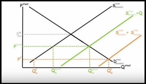
|
- Voluntary Export Restraint
- just like a quota except the government of theEXPORTING
government establishes the quota
- Why would they do this? Because we ask them to.
- Health and safty Regulations
- ME: our textbook calls these a type of nontariff
barrier
- Sometimes they are really just to restrict trade rather
than for health or safety, like Japanese made skis are
safer
- Genetically Modigfied foods are allowed in the United
States but many foreign governments restrict our exports of
such foods. For safety reasons or just to restrict trade?
Other videos
17.1.2 Understanding
Exports in an Open Economy 5:22
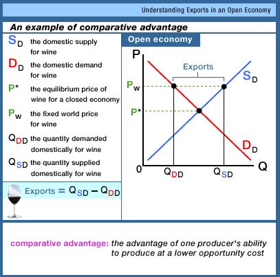
17.3.1 Nominal
Exchange Rates 11:32
17.3.4 Determination
of Exchange Rates 12:31
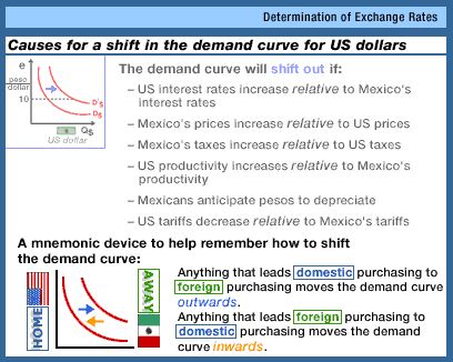
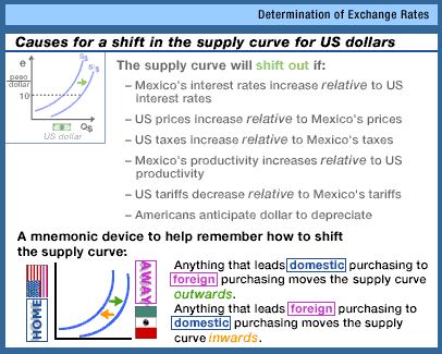
17.3.5 Floating
and Fixed Systems 13:18
Unit 2:
INTRODUCTION TO MACROECONOMICS
|
LESSON12a - Introduction to Macroeconomics and AD
- BUSINESS CYCLES and CIRCULAR FLOW
- AGGREGATE DEMAND
BUSINESS CYCLES
11.1.1 The
Business Cycle Recessions, Depressions, and Booms
2:59
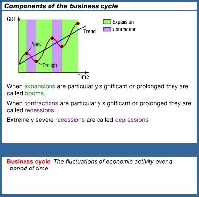
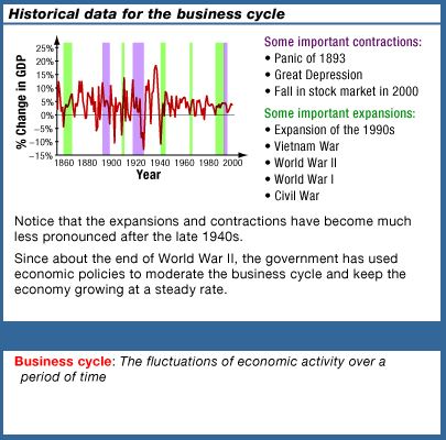
ME: the most recent recession, called The Great Recession,
began in Dec 2007 and ended June 2009
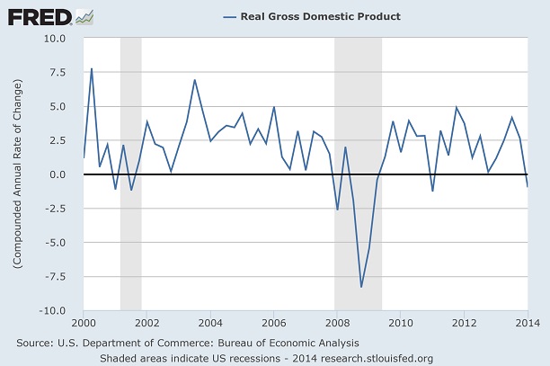
10.1.2 The
Circular Flow Model 9:38
ME: "factors" means "resources"
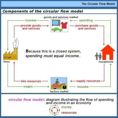
SPENDING = INCOME
Spending must equal income
AGGREGATE DEMAND
14.1.1 Deriving
the Aggregate Demand Curve 7:26
- Aggregate demand (AD) is the sum of all spending in the
economy. We will call this Aggregate Expenditures (AE)
- Well, WHO spends in the economy?
- Consumers (C)
- Business Investment (I) This is business buying capital
resources like factor5eues, this is NOPT finanacial investments
likes stocks and bonds.
- Government purchasing goods and services (G)
- Net Exports (NX in the video,Xn in the textbook) Exports
minus Imports
- Total Spending (AE)= C + I + G + Xn
14.1.2 Movement
along the Aggregate Demand Curve 9:15 [DESCRIBE the
shape of the AD curve]
- Equilibrium in the macroeconomy
- Income = spending
- Y = C + I + G + Xn
- Why does the AD curve slope downwards?
- ME: for all graphs we need to DEFINE, DRAW, and DEFINE.
then we will add DETERMINANTS that shift the curve
- ME: Note how Professor Tomlinson uses Y (income) to measure
output or real GDP
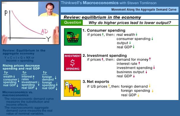
- ME: Our textbook calss these:
- wealth effect
- interest rate effect
- foreign purchases effect
- ME: I wish Professor Tomlinson would use "PL" for the
proice level insteads of just "P", because we used "P" in
chapter 3 to signify the price of just one good. We will always
use "PL" for the macroeconomic Price Level, and "P" for the
microeconomic Price of a single product.
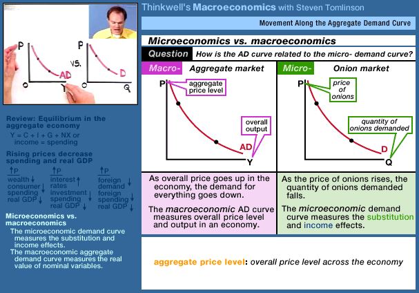
14.1.3 Shifts
in Aggregate Demand 6:03
The SHAPE of the AD curve:
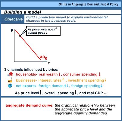
SHIFTING the AD curve

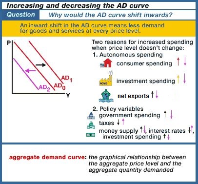
ME: Notice how he shifts the curve LEFT and RIGHT.
ME: see the determinants in the Yellow Pages
LESSON 12b - Aggregate Supply (AS) and
Equilibrium in the Macro-Economy (UE, IN, and EG)
- AGGREGATE SUPPLY
- EQUILIBRIUM
AGGREGATE SUPPLY
14.2.1 The
Short-Run Aggregate Supply Curve 9:03
- How the aggregate quantity supplied is related to the price
level is controversial among economists
- Long run
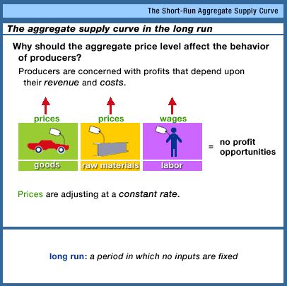
- Short run: prices adjusting at different rates creates an
opportunity for more profit when the price level rises
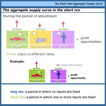
- In the short run there can be confusion and some prices are
sticky
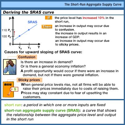
14.2.2 The
Labor Market 7:20
- Three causes of the upward sloping short-run AS curve
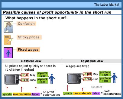
- Why would wages be sticky?
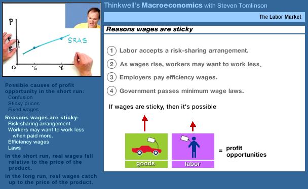
EQUILIBRIUM
14.3.2 Equilibrium
in the Short Run 12:10
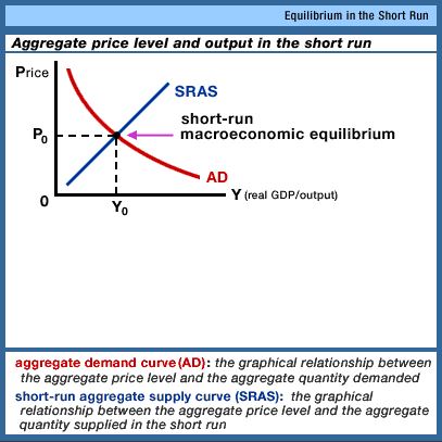
- ME: our textbook states the determinants of AS differently
- change in the prices of resourses
- changes in the productivity of resources
- changes in government regulations (red tape) and business
taxes
- ME: The videos do not discuss how changes in ADE or AS affect
UE, IN, and EG. We will do that in class
14.3.7 Hot
Topic: Oil Shocks 4:52
- ME: These videos were made in the early 2000s (around
2004) when oil price were high. Currently (2015) oil prices are
very low, but the analysis of increasing oil prices can provide
proactice for us in using the AS and AD model and the effects on
UE, IN, and EG.
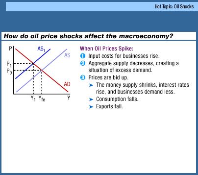
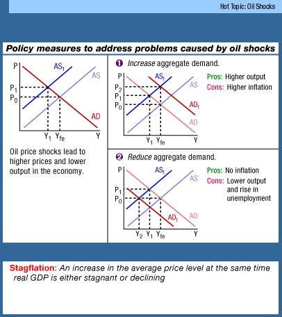
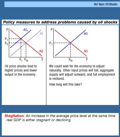
LESSON 12c - Stabilization Policies and AS/AD
in the Long Run
14.2.3 The
Long-Run Aggregate Supply Curve 11:17
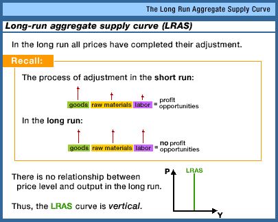
- ME: An increase in the LRAS is economic growth, but
which kind? Achieving our potential or Increasing our
potential?
- It is INCREASING our potential
- What causes this type of economic growth?
- more resources
- beter resources
- better technology
|
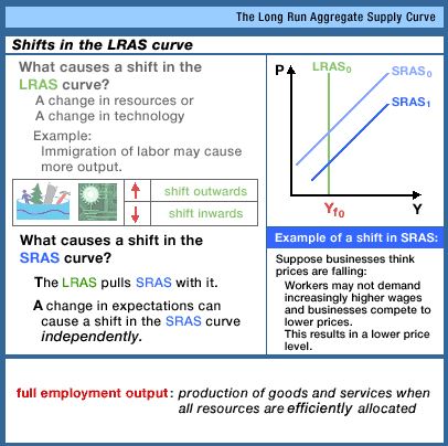
|
14.3.3 Equilibrium
in the Long Run 7:32
14.3.4 Expectations
in the Long Run and the Short Run 14:36
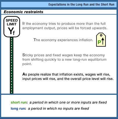
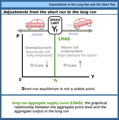
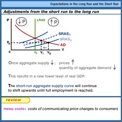
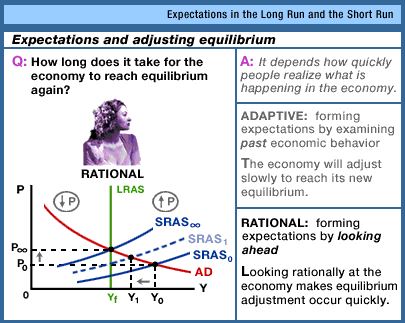
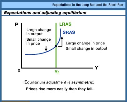
14.3.5 Long-Run
Macroeconomic Equilibrium 16:55
- Three possibilitites are examinined
- an increase in AD
- a decrease in the short run AS (supply shock)
- an increase in the productive capacity of the economy = an
increase in the LRAS
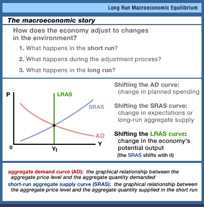
- Short run and long run responses to an increase in AD
- Short run and long run responses to a decrease in AS
- Short run and long run responses to an increase inthe
productive capacity of the economy = an increase in the LRAS
ME: Our textbook's determinants are:
Basically this is more resources, better resources, and better
technology causing an increase in the LRAS
14.4.1 The
Phillips Curve: Definitions and the Historical Record
13:38
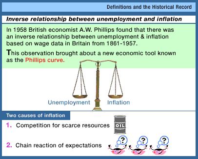
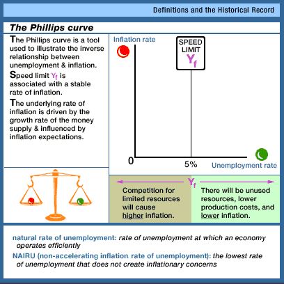
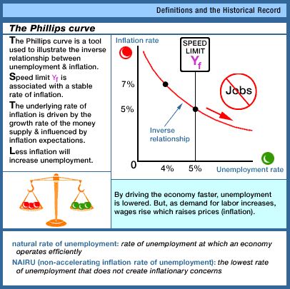
- ME: In the figure above Professor Tomlinson's "underlieing
rate of inflation" at 5% sure seems high to me. He did record
these videos in 2004 so maybe that is why he chose 5%.
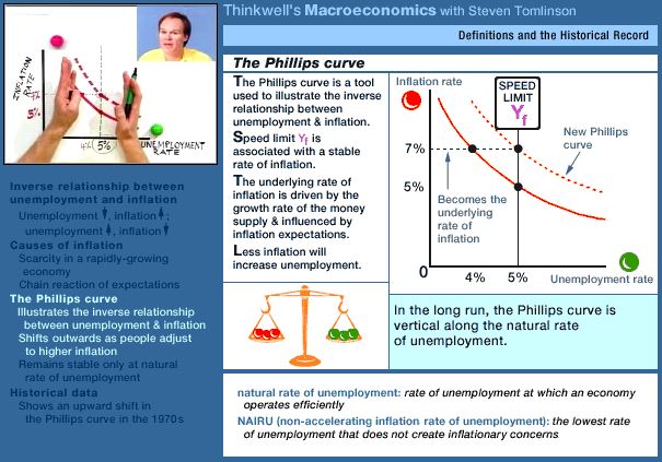
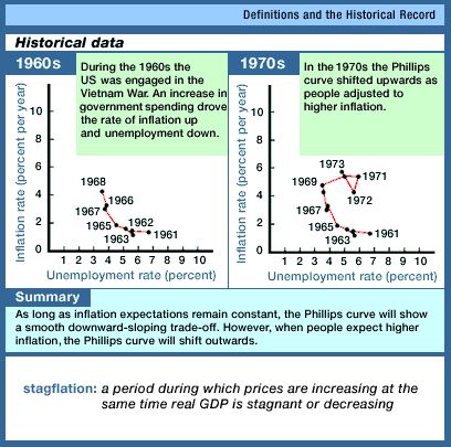
14.4.2 Expectations
and the Phillips Curve 9:15
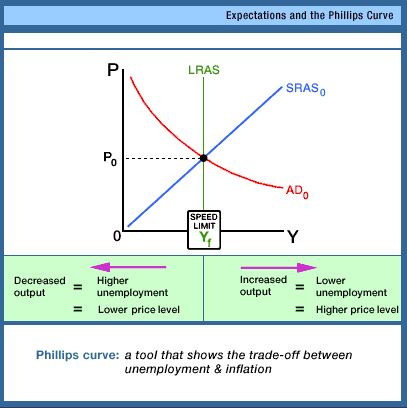
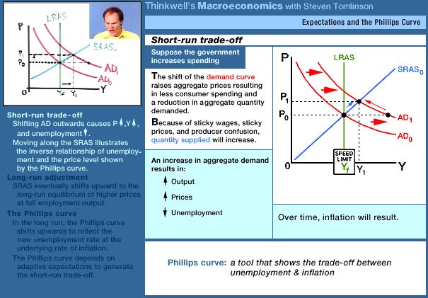
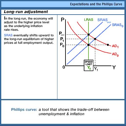
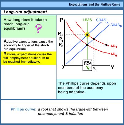
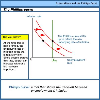
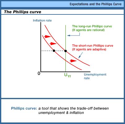
LESSON 9a - Unemployment (UE)
11.2.1 Measuring
the Labor Force and Unemployment 5:48
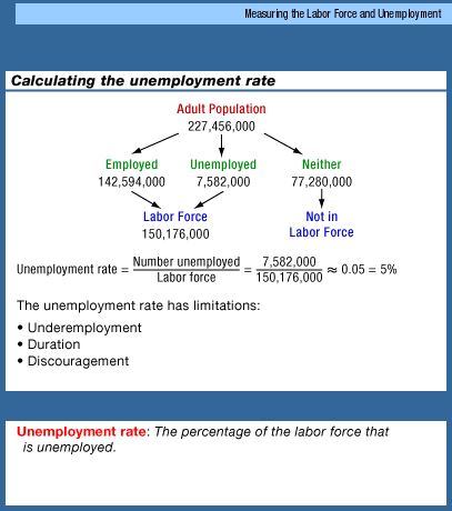
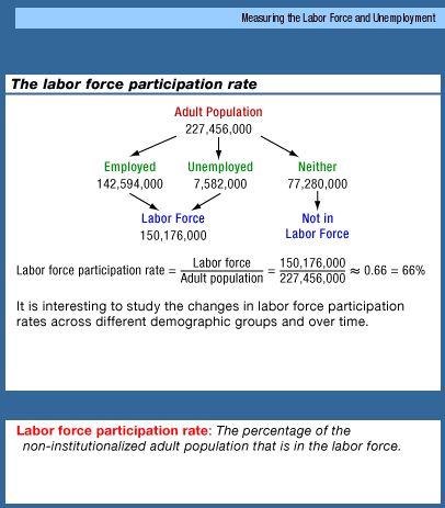
11.2.2 Types
of Unemployment 4:18
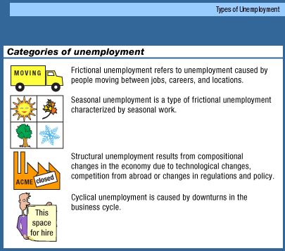
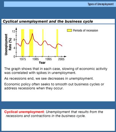
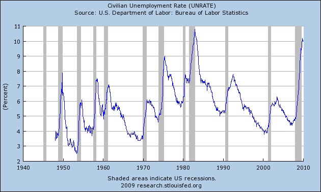
The videos were made in about 2004. The figure above on the
right shows more recent data inclucing the "Great Recession" of
2007-2009.
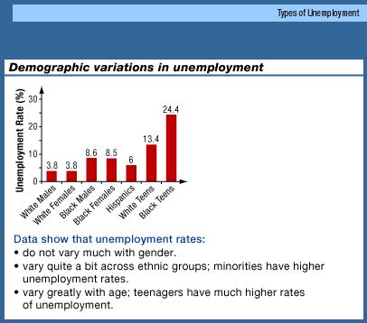
11.3.1 Understanding
the Natural Rate of Unemployment 4:05
ME: The natural rate of UE is about 5%, but it has
changed over time
ME: 5% unemployment then is called Full Employment, or the
"Full Employment Rate of UE" or the "Natural Rate of
unemployment".
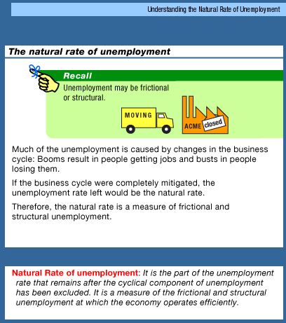
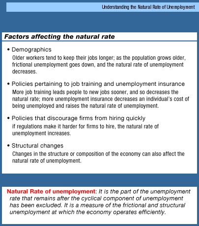
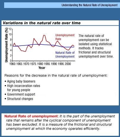
ME: Changes in the full employment rate of unemployment
- 1960's: 4%
- 1970's: 5%
- 1980's: 6%
- 1990's: 5%
- 2000s: maybe 6% (or more)
- around 2015: 5% ?
LESSON 9b - Inflation (IN)
11.5.1 Inflation,
Deflation, Stagflation, and Hyperinflation 4:54
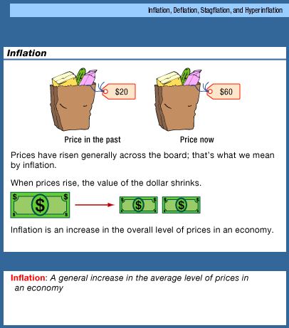
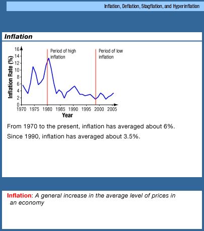
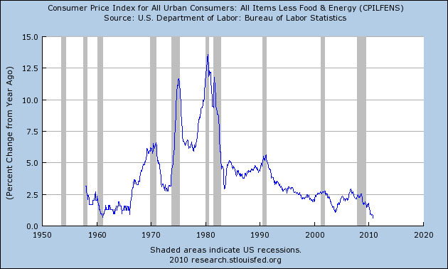
ME: As you can see in the figure above on the right, in more
recent years inflation has been around 2% or less. Also, notice
how during most recessions (the shaded bars) the rate of inflation
falls EXCEPT during the stagflation of the 1970s and early
1980s.
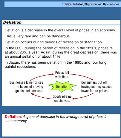
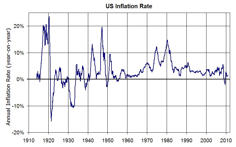
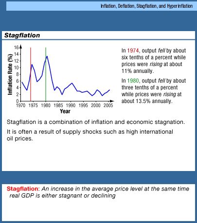
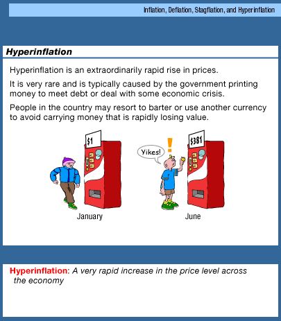
10.3.1 Changes
in the Cost of Living and the CPI 4:47
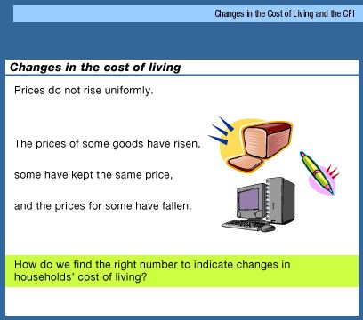
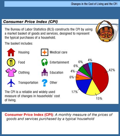
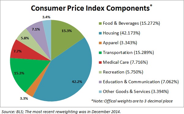
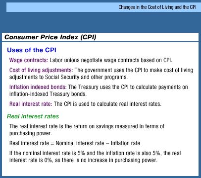
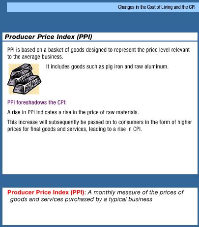
10.3.2 Calculating
the Rate of Inflation 7:33
ME: Please pay close attentin to the CPI and how
tocalculate the rate of inflation with the CPI. We will not spend
much time with the GDP deflator.
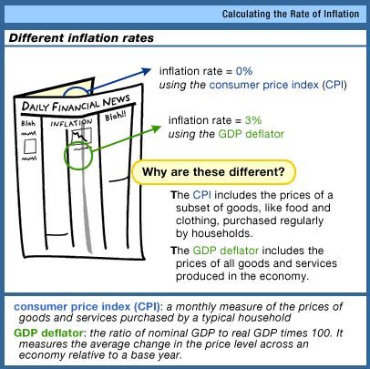
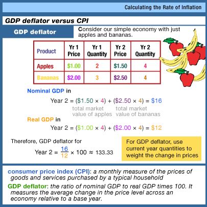
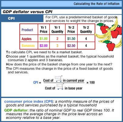
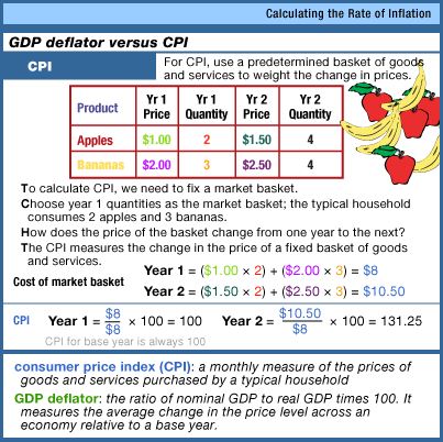
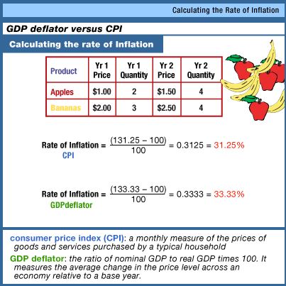
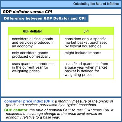
10.3.3 Comparing
the CPI and the GDP Deflator 6:02
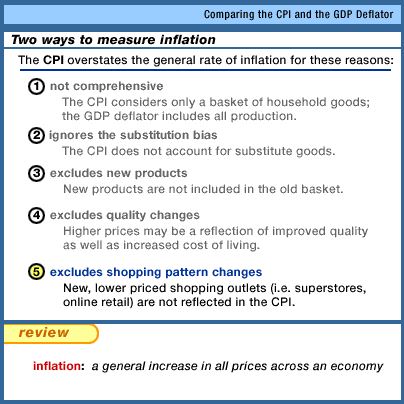
11.5.2 Inflation
and Purchasing Power 7:45
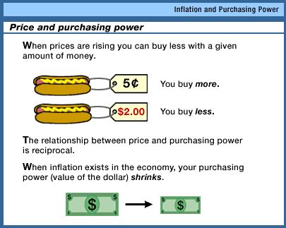
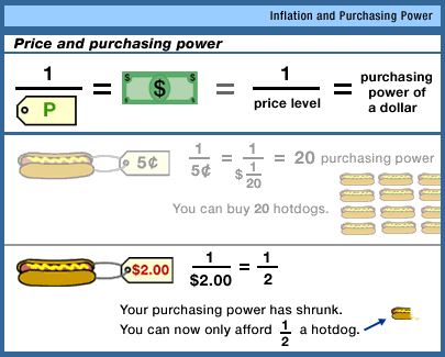
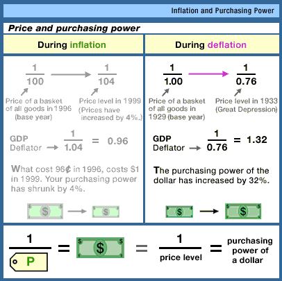
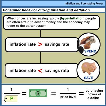
11.5.3 Short-Run
Causes: Demand-Pull and Cost-Push Inflation 9:59
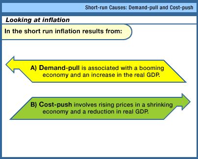
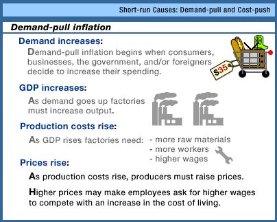
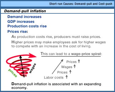
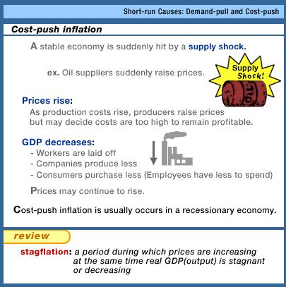
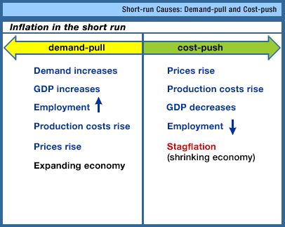
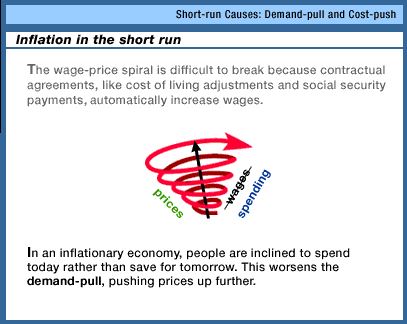
11.5.5 The
Costs of Inflation 9:23
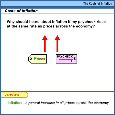
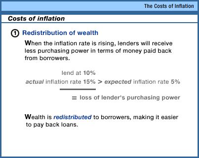
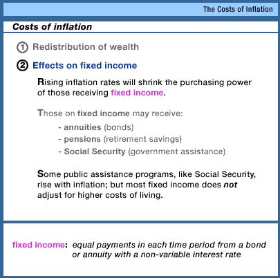
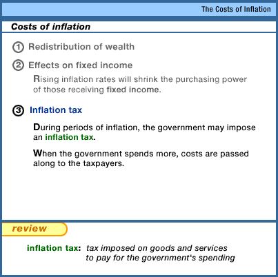
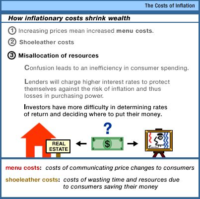
11.5.6 Case
Study: Behavior during Hyperinflation 6:14
LESSON 7a - Measuring the Economy: GDP
10.1.1 REVIEW (1d) The
Production Possibilities Frontier: Macroeconomic
Applications 18:18
- ME: "investment goods" are called "capital goods" in out
textbook (chapter 1)
- ME: Professor Tomlinson uses the term "PPF", our textbook uses
the term "PPC".
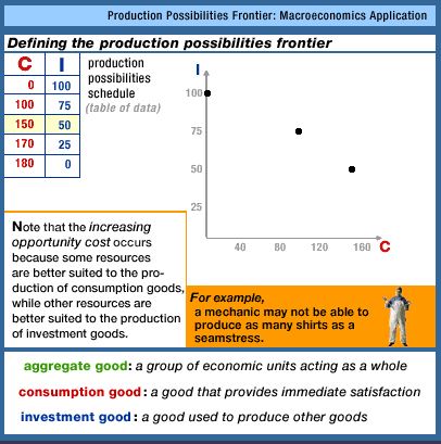
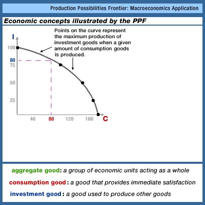
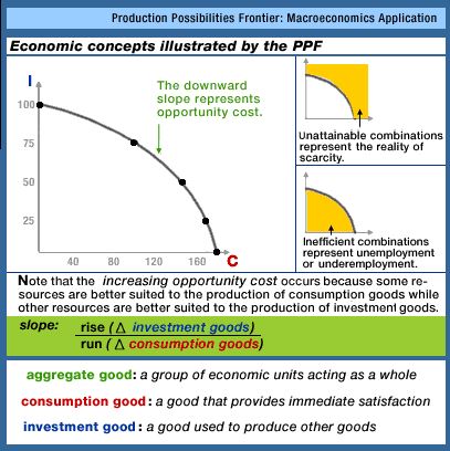
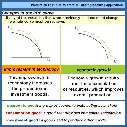
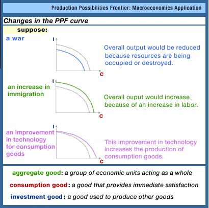
10.1.2 REVIEW (2a) The
Circular Flow Model 9:38
- ME: Professor Tomlinson uses the term "factor markets" while
our textbook use the term "resource markets".
- ME: Professor Tomlinson uses the term "goods and services
markets" while our textbook use the term "product markets".
- SPENDING = INCOME
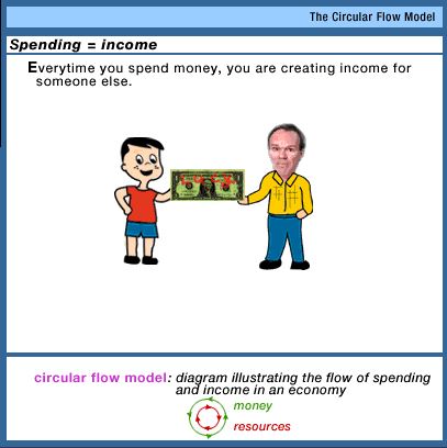
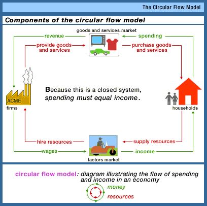
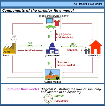
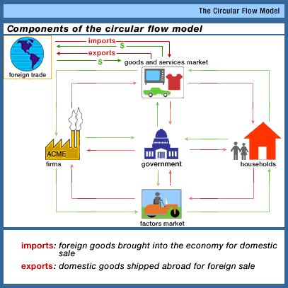
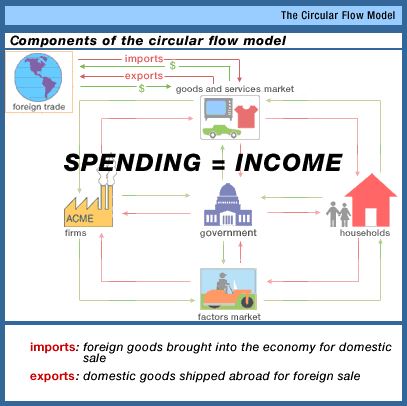
10.1.3 Real
GDP 12:01
- Definintion of GDP
- GDP vs GNP
- nominal GDP vs.real GDP
- ME: What Professor Tomlinson calls a\t "GDP deflator" is
called the "GDP price index" in our textbook
- ME: Real GDP is a measure or real domestic output (RDO) that
we put on our AD/AS graph (horizontal axis)
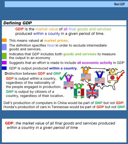
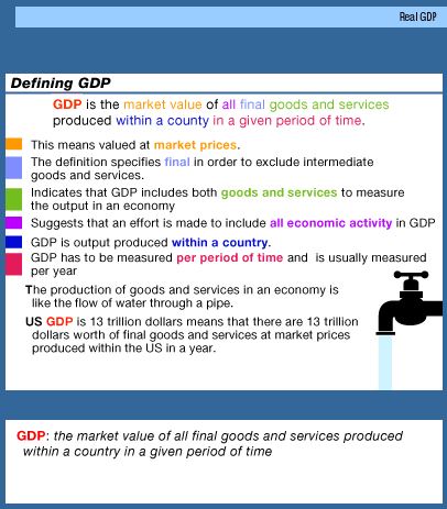
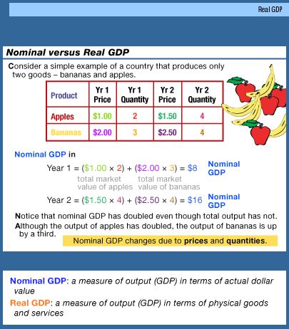
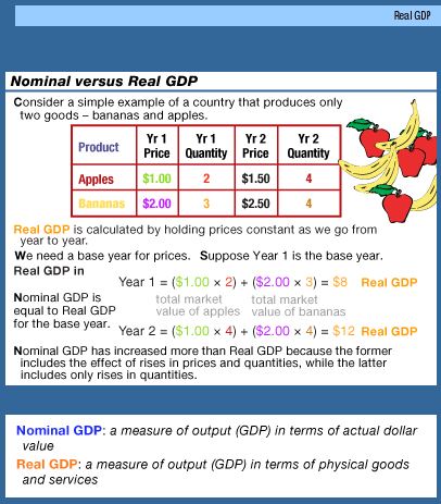
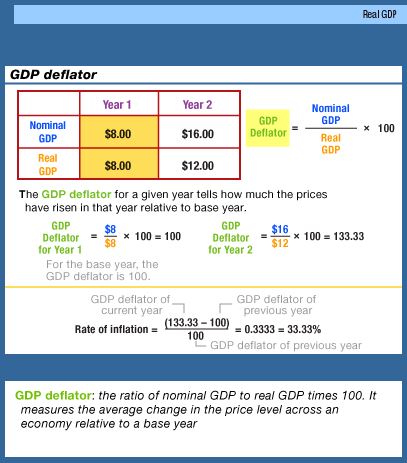
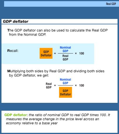
10.1.4 The
BEA Procedure for Calculating Real GDP 8:15
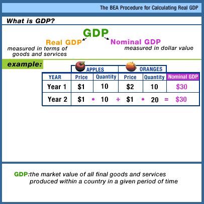
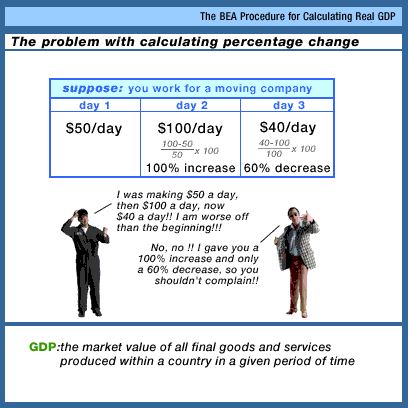
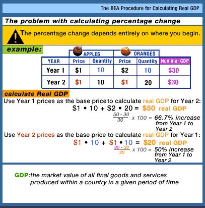
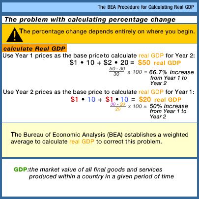
10.1.5 Limitations
of GDP and Alternative Indexes 4:51
ME: From our textbook: Problems with using GDP to Measure
the Standard of Living:
- non-market transactions are not included in GDP
- leisure increases the standard of living but it isn't
counted
- improved product quality often isn't accounted for in
GDP
- GDP does not account for the composition of output
- GDP does not account for the distribution of output
- increases in GDP may harm the environment and decrease the
standard of living
- the underground economy produces goods and services but
they are not included in GDP
- GDP does not account for a possible future decline in
output due to resource depletion.
- Noneconomic Sources of Well-Being like courtesy, crime
reduction, etc., are not covered in GDP.
- We must use per capita GDP to compare the living standards
of different countries.
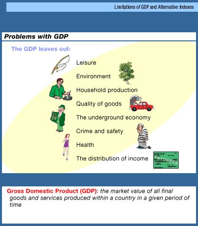
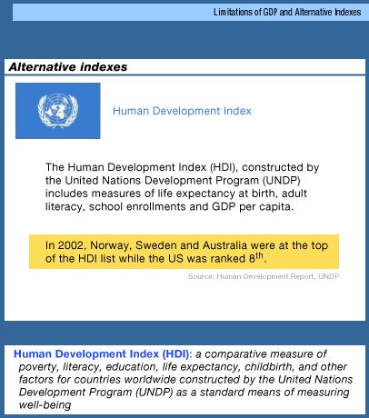
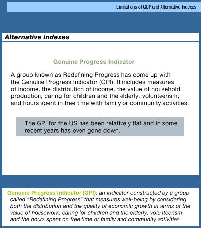
10.2.1 The
Expenditures Approach 4:54
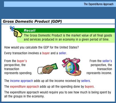
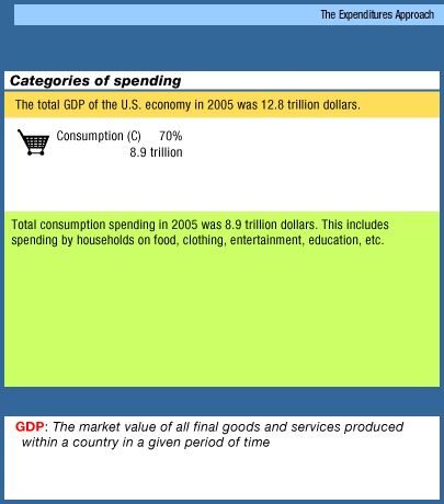
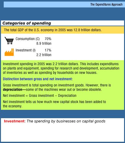
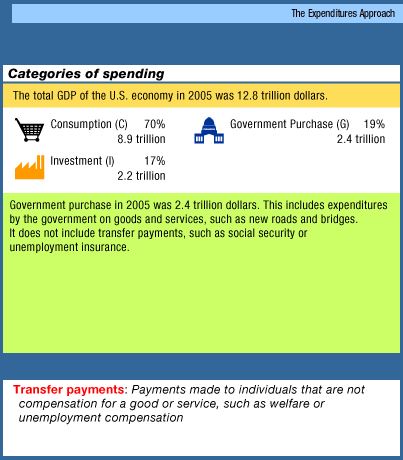
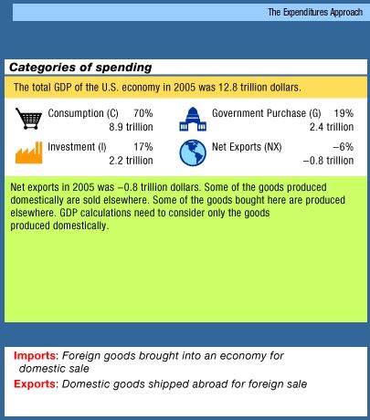
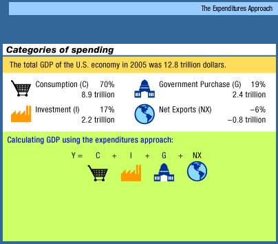
10.2.2 The
Income Approach 7:02
ME: This video is far too complicated which Professor
Tomlinson admits Here is what you need to bwable to calculate:
Required Formulas:
- GDP = C + Ig + G + Xn
- NI = wages + rents + interest + corporate profits +
proprietor's income
- NDP = C + In + G + Xn = GDP - depreciation
- NDP = GDP - depreciation
- In = Ig - depreciation
- Xn = X - M
- real GDP = (nominal GDP / price index) x 100
ME: You have probably noticed already that Professor Tomlinson
uses the letter "Y" to stand for "GDP"
ME: I like to say that
- NI = Income EARNED by the four factors of production
(labor, entrpreneurs, land, and captital)
- PI = Income RECEIVED (unfortunately Prof. tomlinson uses
income "received" for NI)
- DI = SPENDABLE income
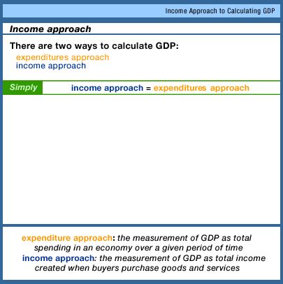
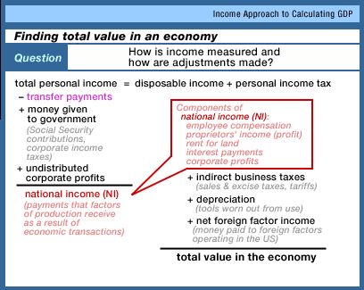
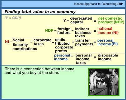
EconMovies-
Episode 6: Back to the Future (Nominal vs. Real, Unemployment,
Inflation) (6:29)
- Macroeconomic issues:
- The original Back to the Future movie was released in
1985
- 1955: EG rate was 7%; Nom. GDP = $415 billion; Real GDP =
$2.78 trillion; UE rate = 4% = full employment; IN rate <
1%
- 1985: EG rate was 4%; Nom. GDP = $4.2 trillion; Real GDP -
$7.7 trillion; UE rate = 7.5%; IN rate = 4%
- 2015:
LESSON 8a - Economic Growth (EG)
16.1.2 The
PPF, the AD/AS Model, and Long-Run Growth 7:44
- ME: our textbook uses PPC (production possibilities curve)
instead of PPF (production possibiities frontier). They are the
same thing.
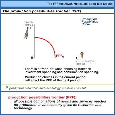
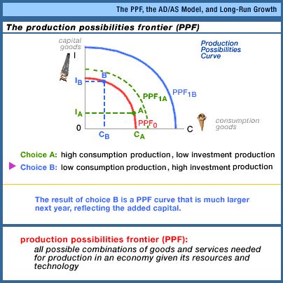
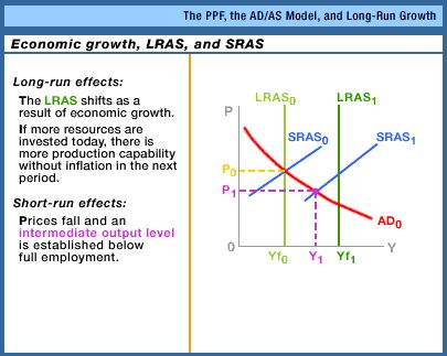
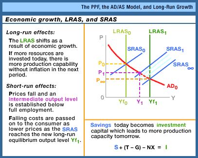
16.1.3 The
Production Function and Growth 6:49
- ME: What professor Tomlinson calls natural resources (N) we
calld LAND in chapter 1 and what he call human capital (H) we
called ENTREPRENEURIAL ABILITY.
- ME: the "production function" is another way to say: "more
resources, better resources, and better technology".
- ME: An "increase in production per worker" means an increase
in labor PRODUCTIVITY which will be defined inhe next video.
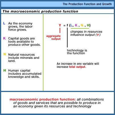
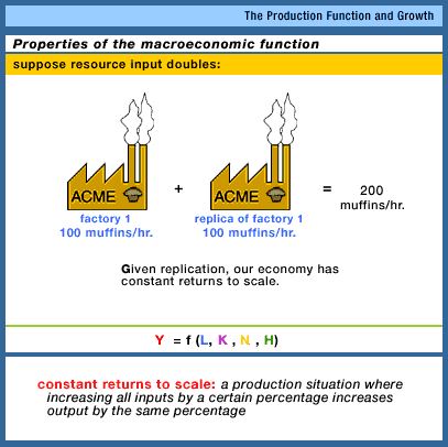
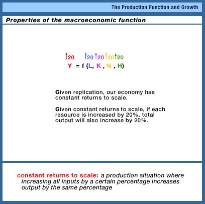
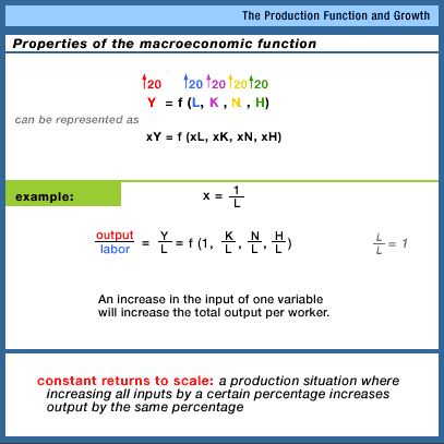
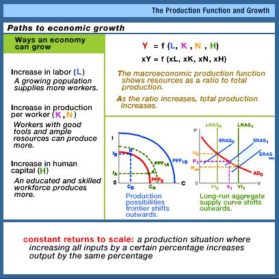
16.1.4 The
Definition of Productivity and Factors Affecting It
3:54
- ME: "Natural Resources" = "land".
- ME: Our textbook lists five factors that affect labor
productivity:
- technological advance [Video: technology]
- quantity of capital per worker [Video:
capital]
- education and training [Video: human
resources]
- economies of scale
- resource allocation
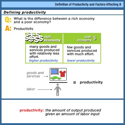
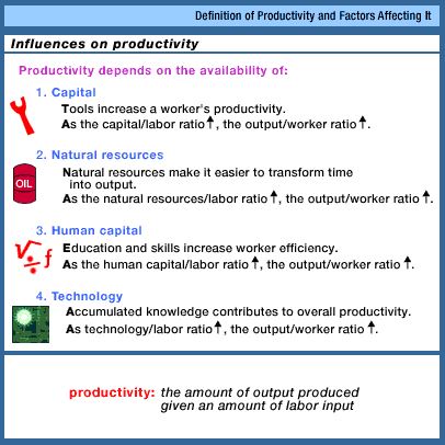
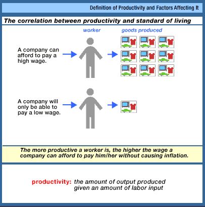
LESSON 22Wa - Growth in the Less Developed
Countries
Videos:
16.3.1 Growth
in Emerging Economies 10:23
- Outline
- Cycle of Poverty
- Ways to break the cycle
- better financial institutions
- technological progress
- government stimulation
- population control (?)
- China and India
- China-industirialization; India-services
- Challenges
- Cycle of Poverty: Why do some countries become rich while
others are stuck in poverty? The field of Development Economics
- low per capita GDP (low incomes) CAUSE
- low savings and demand which CAUSE
- low investments which CAUSE
- low productivity which CAUSES
- low per capital GDP (low incomes)
- ME: be sure you know the economic definition of
INVESTMENT.
- It IS NOT the stock market
- it IS businesses buying more factories,
machines, tools, etc (buying more captital)
- ME: note the central roll plyed by saving,
investment, and productivity
|
|
- low incomes and poorly developed finanacial
institutions cause low savings therefore there are few
funds available for businesses and governments to
borrow to make investments in capital and
infrastructture
- low savings = low investment
- low investment = low productivity = low
incomes
|
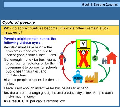
|
- Ways to break the cycle
- try to get people to save more by providing better
financial institutions; even poor people can save if
they have good banks, etc.
- improving technology to improve productivity
- government can play a role by:
- improving finanacial institutions
- stimulate demand to boost incomes and then
savings
- borrow from international institutions to
improve infrastructure which will increase
productivity
- reduce population growth rates (often
ineffective and controversial)
- children are often seen as a type of social
security - someone to care for you in old
age
- when economies grow, birth rates tend to
decrease
|
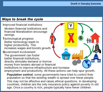
|
- China and India
- together comrise 1/3 of the world's
population
- both have rapidly growing economies
- but there are differences
- China has been growing faster than India
- China: manufacturing sector
- India: services sector
- China began earlier using newly developed supply
chains basied on manufacturing and trasportation
technologies
- India's depended on communication technology that
developed latter
- China has had amazing increases in its standard of
living
- ME: China pulled 680m people out of misery in
1981-2010, and reduced its extreme-poverty rate
from 84% in 1980 to 10% now
- Challenges and Prospects
- unemplouyment
- problems transforming from agriculture to
industry
- political tensions and challeges from
neighbors
- pollution
- health problems
- future population growth
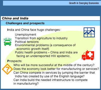
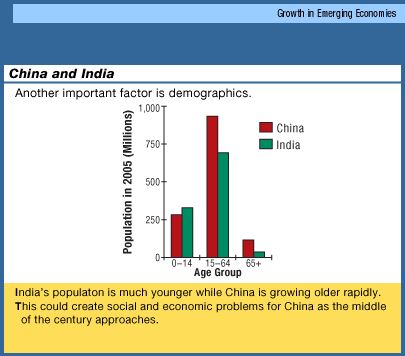
|
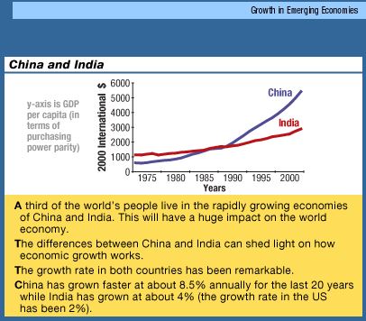
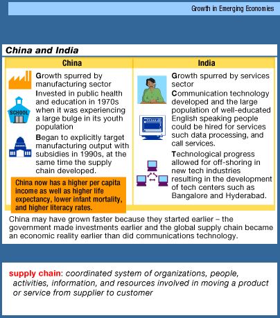
|
10.1.6 The
Growth of China as a Superpower 2:14
- Outline
- Interesting facts about China's rapid economic
growth
- Chinga's economy has grown at about 7.5% a year since
1984
- China now (2004) produces 12% of the total world
output (2014: 16%)
- Consequences of rapid growth
- increased pollution
- increase in the standard of living
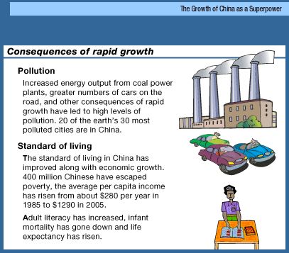
16.3.2 Policies
to Promote Growth 7:50
|
Outline
- Government Policies
- Breaking the Gycle
- transition from agricultural evconomy to
industrial economy
- stimulate export demand
- transtion from a centrally planned economy to a
free market ecoamy
- ME: NOTE - the video has this backwards on
its outling under Tomlinson's picture
- World Bank and the IMF
- What are they?
- Debate about whether they are
effective
|
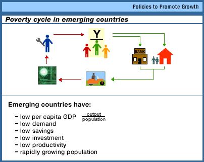
|
ME: From our textbook:
- Positive Role of Government in Promoting Growth
- Establishing the rule of law
- Building infrastructure
- Embracing globalization
- Building human capital
- Promoting entrepreneurship
- Developing credit systems
- Controlling population growth
- Making peace with neighbors
- Public Sector Problems
- misadministration
- corruption
|
Video: The video seems to look at older policies BEFORE
the movement to Structutral Adjustment
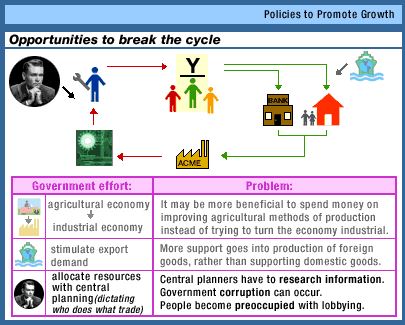
|
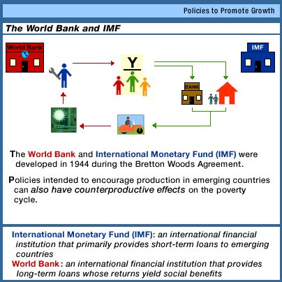
16.2.2 Other
Policies to Encourage Growth 10:40
- ME: good discussion about population growth and economic
growth
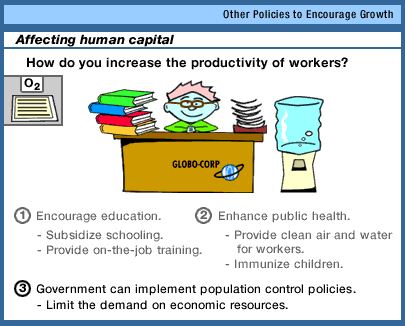
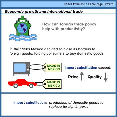
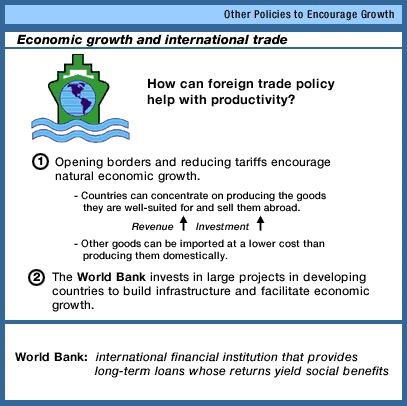
16.3.3 Hot
Topic: The Myth of Exploding Populations 8:00
Mlthus thought that since population grew geometrically and
food production gre arithmatically eventi=ually popltion growth
would overtake food production and there would be massive famine.
See below on the graph at the right. When population is greater
than food production famine will occur.
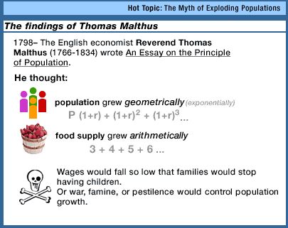
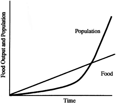
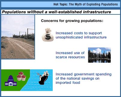
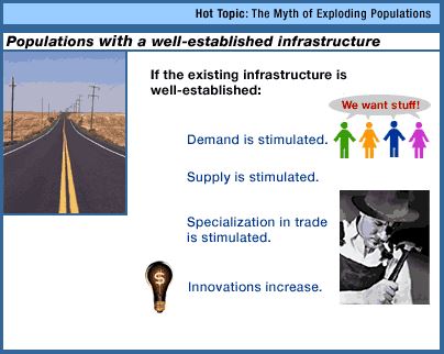
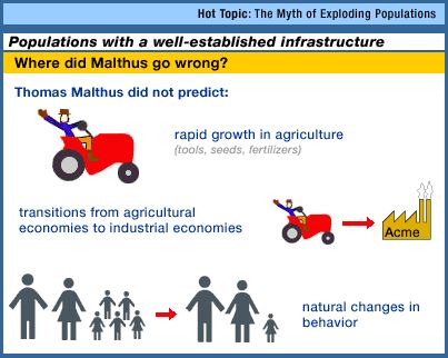
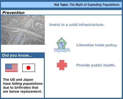
16.2.3 Hot
Topic: Women's Roles in Rural Economic Growth 4:59
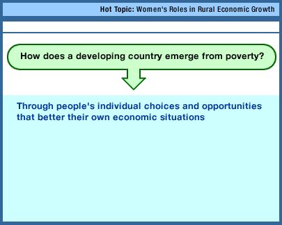
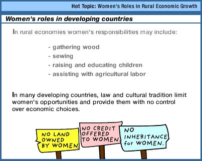
Unit 3: MACROECONOMIC
POLICY
|
MONETARY POLICY
LESSON 14a - Money, Money Market, and the
Fed
13.1.1 The
Money Supply 8:10
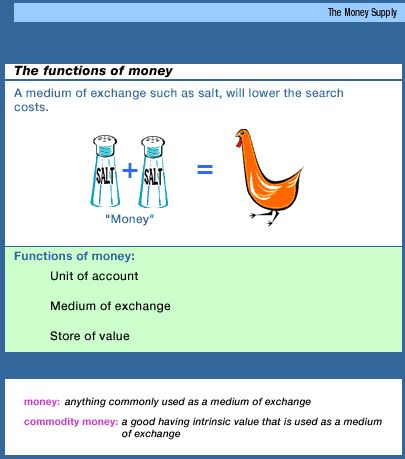
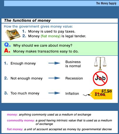
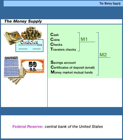
13.4.2 Case
Study: Cigarettes As Money 6:07
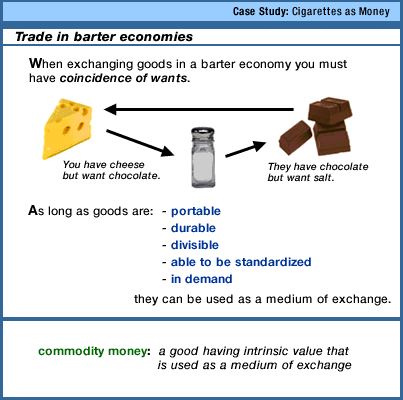
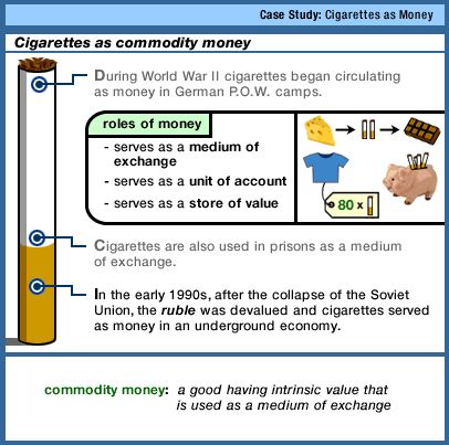
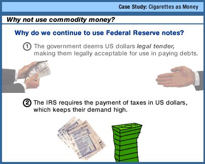
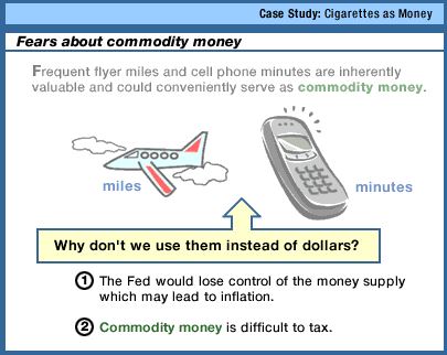
13.1.2 Determinants
of Money Demand 9:00
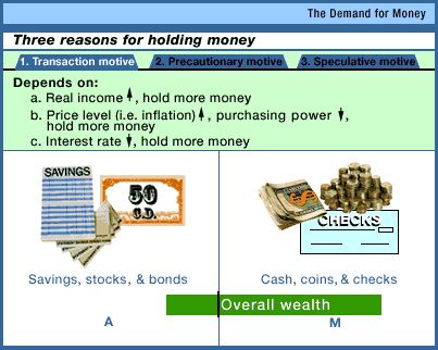
ME:: our textbook says (p. 315) that we will keep it simple and
ssume that the transactions demand for money only depends on
nominal DP which is really ther same as real income and the price
level. So, we will NOT say that the transactions
demand for money is inversely related to the interest rate. in
other words we will assume that the transactions demand for money
is independent of interest rates (see graph above).
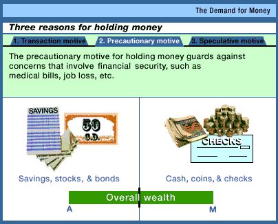
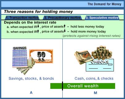
ME: Our textbook combins the precationary motive and the
speculative motive into the "asset demand" for money. Although the
video and textbook approaces money demand a bit differely, they
got to the same result: a dowanrd sloping money menand (total
money demand) curve.
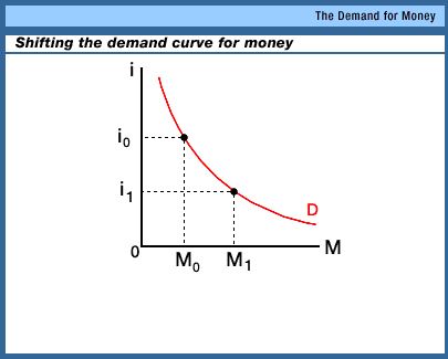
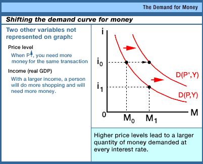
ME: The video says that higher price levels or higher real
income will increase money demand. Out textbook says that higher
nominal income (nominal GDP) will increase money demand. these are
really the same thing since: nominal income = real income times
the price level.
13.1.3 The
Money Market 10:02
The equilibrium interest rate is where the money demand
curve crosses the money supply curve (see graphs below).
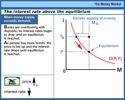
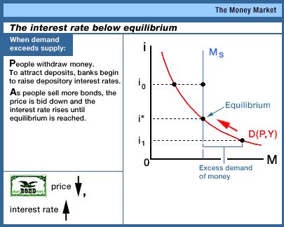
What then will change interest rates? Well. a change in money
demand or a change in money supply will cause interese rates to
change (see graphs below).
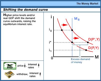
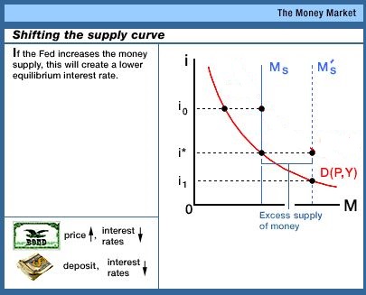
ME: We will pay most attention to changes in the money supply
(MS)
REMEMBER: a change in the MS CAUSES a change in interest rates,
NOT: a change in interest rates causing a change in the MS.
AC Money
Market - Macro Review 3:24 [YouTube
ACDCLeadership]
13.3.1 The
Federal Reserve System 8:13
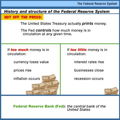
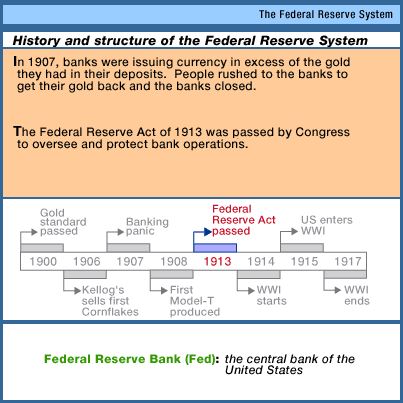

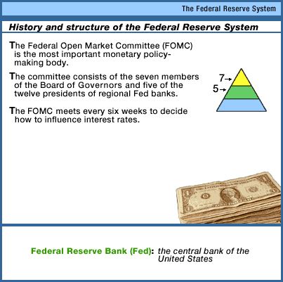
ME: The current chair of the Fed is JJerome Powell who took
office in February 2018.
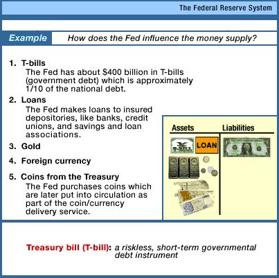
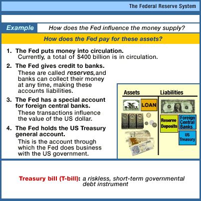
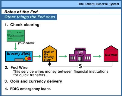
ME Functions of the Fed from our textbook:
1. issue currency = Federal Reserve Notes
2. setting reserve requirements or reserve ratios (RR see
chapter 16)
3. lending money to banks and thrifts (the discount rate -DR-
is the interest rate banks are charged for borrowing from the
Fed)
4. providing for check collection
5. acting as fiscal agent for the US government
6. supervising banks
7. controlling the money supply
ME: Currently the Fed owns about 14% of the US debt or about
$2.5 trillion.
LESSON 15a - How Banks Create Money
13.4.1 How
Goldsmiths Created Money 7:40
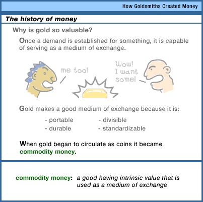
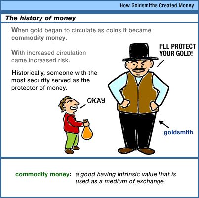
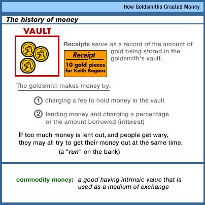
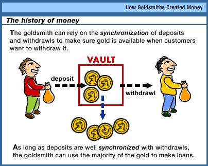
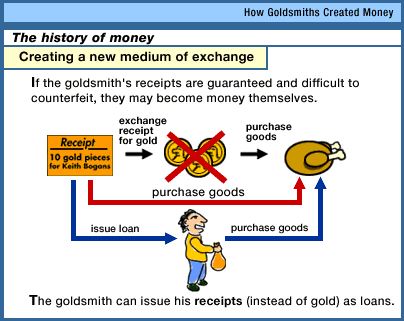
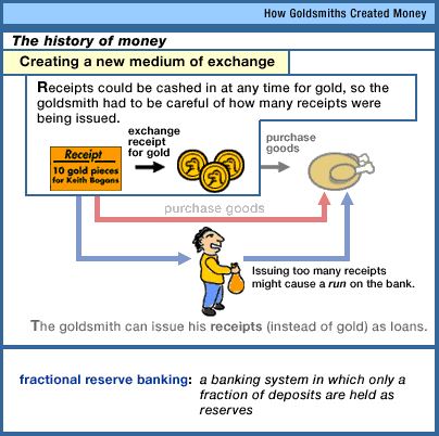
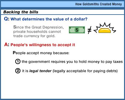
ME: Our textbook says that a dollar has value because of
- accepability
- legal tender
- relative scarcity
13.4.3 How
Banks Create Money 12:09
Professor Tomlinson does this a little bit differently
than we will and he makes either an error or an
oversimplification, or he is doing something that we will do in
chapter 16. Either way it cam be a little bit confusing. Still, I
like how he goes thorugh the money multiplier process. It is just
like I have been doing it (except for his one error).
He says: Change in MS = change in deposits x the money
multiplier
We say: Change in MS = Initial excess reserves x Money
Multiplier
If you look at the "notes"
that are available on the Thinkwell video site (Click on "Chapter
Checklist" or click HERE)
the notes do it the way we do it
What the videos calls "Lendable Reserves" our textbook calls
Excess Reserves (ER). (See his "notes")
Formulas from the yellow pages:
- Total Reserves = Cash in vault + Deposits at Fed
- Required Reserves = RR x Liabilities
- Excess Reserves = Total Reserves - Required Reserves
- Money Multiplier = 1 / RR
How
banks create money and the money multiplier 4:12
YouTube ACDC Economics)
LESSON 16a - Monetary Policy (MP)
13.3.3 The
Fed's Tools of Monetary Policy 9:46
Alan Greenspan was Chair of the Fereral Reserve board of Governors
from 1987 to 2006. Janet L. Yellen took office as Chair of the Board
of Governors of the Federal Reserve System on February 3, 2014, for a
four-year term ending February 3, 2018. Dr. Yellen also serves as
Chairman of the Federal Open Market Committee, the System's principal
monetary policymaking body. Prior to her appointment as Chair, Dr.
Yellen served as Vice Chair of the Board of Governors, taking office
in October 2010, when she simultaneously began a 14-year term as a
member of the Board that will expire January 31, 2024.
When a bank makes a loan they create checking account deposits
(also called "Demand Deposits"). These deposits are NEW MONEY. The
Fed controlls how many loans (how much money) banks can create.
The Fed has three tools to control the MS.
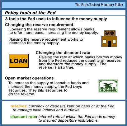
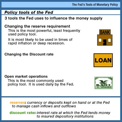
Professor Tomlinson says that the Fed controlls the MS by
controlling bank RESERVES. This, of course, is correct, but it is
more correct to say that the fed controls the MS by controlling the
EXCESS RESERVES of banks. This is how our textbook explains monetary
policy.
13.4.4 How
the Fed Changes the Money Supply 10:06
This video repeats part of the previous, but it is a good review,
and more information is added.
15.4.3 Monetary
Responses to Changes in the Economy 12:20
AC Macro
4.1- Money Market and FED Tools (Monetary Policy) 5:20
[YouTube ACDCLeadership]
AC Macro
4.9- Monetary Policy Practice 3:21 (recessionary gap)
[YouTube ACDCLeadership]
AC Macro
4.10- Graphing Monetary Policy Practice (AP Macroeconomics) 2:44
(inflationary gap) [YouTube ACDCLeadership]
15.4.3 Monetary
Responses to Changes in the Economy 12:20
OPTIONAL 13.3.4 Case
Study: The Greenspan Era 3:16
LESSON 16b - Other Monetary Policy
Issues
OPTIONAL 11.1.2 Theoretical
Explanations for Cycles 10:09
11.5.4 The
Quantity Theory of Money 11:58
What Professor Tomlinson calls the "Quantity Throey of
Money", our textbook calls the "Equation of exchange"
What Professor Tomlinson calls Y (income) our textbook calls Q.
Both mean the same thing: real GDP or output in the economy.
15.5.1 New
Keynesians versus Monetarists 11:23
"New Keynesians" are also called "Mainstream economists"
in our textbook.
Video: MV = PY
Textbook: MV = PQ
They are the same thing.
15.5.2 New
Classical Macroeconomics 8:31
15.5.3 Case
Study: Policy in the Great Depression 8:22
Established in 1933 and repealed in 1999, the Glass-Steagall
Act
15.4.5 Hot
Topic: Should Monetary Policy Be Made by Rule or
Discretion? 5:03
MJM 25 Macroeconomic
Viewpoints 7:06 [YouTube mjmfoodie]
FISCAL POLICY
LESSON 10a - The Spending Multiplier
15.1.1 Recessions
and Booms Unanticipated Changes in Aggregate Demand
12:04
Notice how Prof. Tomlinson discusses how the real GDP (Y)
adjusts to the decrease in demand by using the factors that
explain why the AD curve is downward sloping: (1) wealth effect,
(2) interest rate effect, and (3) foreign purchases effect.
15.1.2 Recessions
and Booms Unanticipated Changes in Aggregate Supply
15:43
Remember, these videos were made around 2004, so when Prof.
Tomlinson says that this is what is happening today he means around
12004-2005. BUT, in 2015 I think the economy is similar to what it
was then. so it applies to today as well.
EC Fiscal
Policy – the Government Spending Multiplier
20:07
This video assumes that the price level is not changing.
therefore any change in AD is an equal change in real GDP.
The speaker does mention the "complex multiplier" at the end of
the video (although he does not use that term) when he mentions
that their are other leakages fromthe economy besides just
savings. Since there are more leakages the complex mutiplier will
be smaller than the government spending (or simple
multiplier).
Simple multiplier = government spending multiplier = 1/1-MPC =
1/MPS
Complex multiplier = 1/all marginal leakages =
1/MPS+MPM+MPT
MPS is the marginal propensity to save = the fraction of
addition income that is saved
MPM is the marginal propensity to spend on imports = the
fraction of additional income that is spent on imports
MPT is the marginal propensity to tax = the fraction of
additional income that is used to pay taxes
AC Macro
3.9- Multiplier Effect, MPC, and MPS 2:17
AC Macro
3.10- Calculating the Multipliers 1:50
AC Macro
3.11 Multiplier and Spending Practice 2:02
Major error or oversimplification:
Mr. Clifford should have a horizontal AS curve when he is doing
these problens. In our next lesson we will learn that the
multiplier with increases in the price level is smaller than the
simple muyltiplier.
As we learned in the 20 minute EconClassroom video above, the
multiplier tells us how much the AD will shift. You can see on the
graph below that Mr. Clifford shifted the AD curve a lot more than
$40.
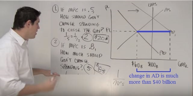
You only get the full effect of the multiplier if the price
level stays constant (if the AS is horizontal. This is how he
should have drawn the graphs. Now the AD curve shifts to the right
by $40 billion and real GDP goes up by $40 billion because there
is no change in the price level.
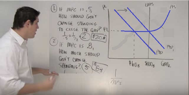
So, if there is an increase in the price level then the
multiplier is smaller. So if we used Mr. Clifford's graph we woul
have to increase government spending (G) by a lot more than
$20 billion (if MPC=0.5) or by a lot more than $8 billion if MPC
is 0.8.
LESSON 13a - Fiscal Policy
- FISCAL POLICY: THE MAINSTREAM
FISCAL POLICY OTHER
FISCAL POLICY: THE MAINSTREAM
15.2.1 Fiscal
Policy Using the AD/AS Model 5:24
A good introduction to some of the issues that we will learn when
we study fiscal policy.
EC Fiscal
Policy – the Tax Multiplier 13:35
The tax multiplier will always be one less than the simple
multiplier but negative. So, if MPC = 0.4 then MPS = o.6 amd the
simple multiplier is 1/MPS = 1/0.6 = 1.67. The tax multiplier then is
just 0.67 or one less than the simple multiplier.
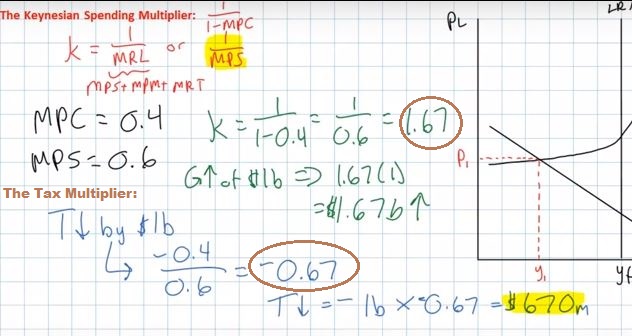
Dr. Welker should have his AS curve horizontal since he ignores
changes in the price level. He is assuming that the price level does
not change. As you can see on his graph below on the left he actually
increases AD by more than $500. He should have drawn his AS curve
horizontal like the graph below on the right. He forgot that if the
price level increases then the multiplier effect is smaller.
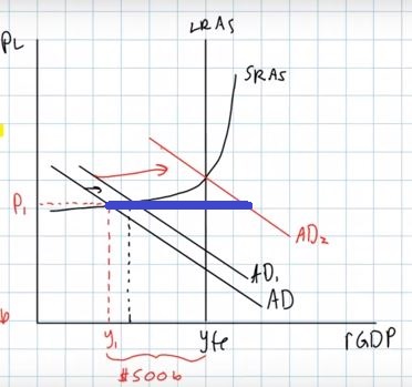
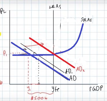
AC Macro
3.12 Multiplier and Taxes Practice 3:20
Again, Mr Clifford is ignoring the effects of an increase in the
price level on the size of the multiplier.
EC Fiscal
Policy – the Crowding-out Effect 14:05
|
The video discusses how the crowding out effect might be
very great and actually cause the mutltiplier to be less
than 1. In other words and increase in G of $100 billion
will cause real GDP to increase by LESS THAN $100.
Our textbook says "An expansionary fiscal policy (deficit
spending) may increase the interest rate and reduce
investment spending, thereby weakening or canceling the
stimulus of the expansionary policy."
In other words the multiplier will be less than the
government spending multiplier, but there could still be a
multiplier effect, only smaller.
|
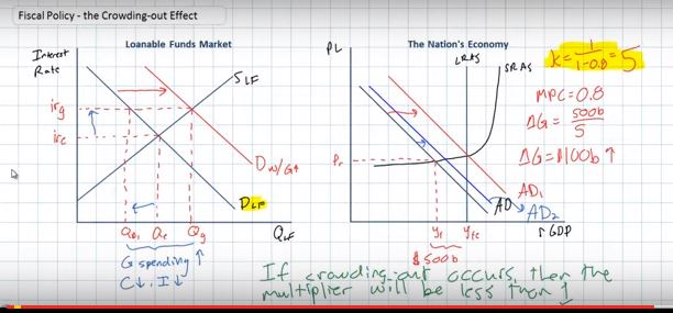
|
More from the textbook not covered in the video:
"Economists vary in their opinions about the strength of the
crowding-out effect. An important thing to keep in mind is that
crowding out is likely to be less of a problem when the economy is in
recession, because investment demand tends to be weak. Why? Because
output purchases slow during recessions and therefore most businesses
end up with substantial excess capacity. As a result, they do not
have much incentive to add new machinery or build new factories.
After all, why should they add capacity when some of the capacity
they already have is lying idle?
With investment demand weak during a recession, the crowding-out
effect is likely to be very small. Simply put, there is not much
investment for the government to crowd out. Even if deficit spending
does increase the interest rate, the effect on investment may be
fully offset by the improved investment prospects that businesses
expect from the fiscal stimulus.
By contrast, when the economy is operating at or near full
capacity, investment demand is likely to be quite strong so that
crowding out will probably be a much more serious problem. When the
economy is booming, factories will be running at or near full
capacity and firms will have high investment demand for two reasons.
First, equipment running at full capacity wears out fast, so firms
will be investing substantial amounts just to replace machinery and
equipment that wears out and depreciates. Second, the economy is
likely to be growing overall so that firms will be heavily investing
to add to their production capacity to take advantage of the greater
anticipated demand for their outputs."
15.2.3 Timing
Problems and the AD/AS Model 6:58
Professor Tomlinson, for some stange reason, doesn't discuss the
multiopliers in his fiscal policy videos. He should have mentioned
that the Operational lag does not only include the time to complete
the government spending programs (like building highways) but it also
includes the time it takes ofr the multiplier to have its full
effect. The road construction workers will spen mote at local bars.
As a result, he local bar owners will see their incomes increase and
they may buy more bar stools, The owners of the furniture company
building the new stools wiill see their incomes increase and maybe
buy a new car. Etc. All of this additional spending and production
takes time. This time is called the operational lag of fiscal
policy.
15.2.4 Automatic
Stabilizers 8:40
When Prof. tomlinson says "automatic stabilzers", our textbook may
say "built-in stabilizers".
Out textbook uses the word "recovery" where Prof. Tomlinmson uses
the word "boom".
15.4.4 Monetary
Policy: Accommodation 9:40
It is interesting that Prof. Tomlinson discusses accommodation by
beginning at the full employment level of output and then increases
AD. What if we were in a recession and the government uses
expansionary FPO to increase AD. We said earlier that government
borrowing will increase interest rates and cause crowding out of
investment wich may reduce the size of the mulitplier and make fiscal
policy less effective. MP accommodation will keep interest rates
lower andreduce the amount of crowding out thereby increasing the
size of the multiplier.
FISCAL POLICY OTHER
15.2.5 Hot
Topic: The Political Business Cycle 3:35
15.3.2 Supply-Side
Policy 5:26
Prof. Tomlinson draws the Laffer curve a bit diffeerently than
does our textbook. He puts tax reveue on the vertical axis whereas
our textbook puts tax revenue on the horizontal access.
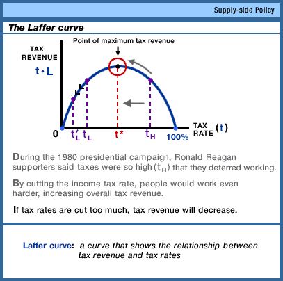
LESSON 13b - Other Fiscal Policy Issues and
Government Debt
15.5.3 Case
Study: Policy in the Great Depression 8:22
15.3.1 New
Keynesian and New Classical Approaches to Fiscal Policy 11:03
17.4.1 Government
Budget Deficits and Trade 5:11
14.3.6 Case
Study: The U.S. National Debt 8:00
The video says the national debt is $7.2 trillion but
that ws in about 20014, currently it is about $17 trillion.
The video says the debt as a % of GDP is 64% but that ws in
about 2004, currently it is about 100%.
NOTE: the video uses the TOTAL debt, not the PUBLIC debt.
Understanding
the National Debt and Budget Deficit (6:33 YouTube
vlogbrothers)
America's
Debt Crisis Explained (5:05 youTube PragerU)