Instructor Notes from the Video
Lectures
The textbook and the online video lectures are written by
different authors and sometimes (often?) different economic
authors use different terminology or different approaches to
discuss the same concept. This webpage will help you see the
connections between our textbook and the online video lectures.
Also, this webpage will allow me to add some of my own comments
and explanations.
You should refer to this page when watching the videos. For the
related textbook readings and other activities see: http://www.harpercollege.edu/mhealy/eco211f/micassigna.htm
Don't forget the quizzes, transcripts, and lecture notes
that accompany most of the video lectures. These can be very
helpful.
UNIT 1
Chapter 1: An introduction to Economics (Modules
1a, 1b, 1c, and 1d)
MODULE 1b - THE 5Es OF ECONOMICS and BASIC MATH
SKILLS
Videos are usually between 5 and 10 minutes long and most of them
have a written transcript available and a multiple choice question
review quiz.
Instructions on how to purchase and access the video lectures can be
found in our syllabus.
- REVIEW OF GRAPHING CONCEPTS
- 1A.1 Using Graphs to Understand Direct Relationships
[TW 1.2.1 (9:50)]
- 1A.2 Plotting A Linear Relationship Between Two Variables
[TW 1.2.2 (9:57)]
- 1A.3 Changing the Intercept of a Linear Function [TW
1.2.3 (8:42)]
- 1A.4 Understanding the Slope of a Linear Function [TW
1.2.4 (7:28)]
- OPTIONAL:
- OPTIONAL: SIMPLE MATH, ALGEBRA, AND GEOMETRY FOR ECONOMICS
STUDENTS
REVIEW OF GRAPHING
CONCEPTS
1A.1 [TW 1.2.1
(9:50)] Using Graphs to Understand Direct Relationships -
1b
- Outline
- How do graphs work?
- About this graph
- How do graphs work
- economists use graphs to represent the relationship between
two variables (sometimes three) in a two-dimensional space
- Example: the relationship between consumption and income
- income on horizontal axis and consumption on the
vertical axis
- ALWAYS LABEL THE AXES
- calibrate the axis with numbers
- put data points on the graph; every point on a graph
represents two numbers
- (horizontal, vertical); (x,y); (30,40)
- About this graph
- the x-axis is horizontal
- the y-axis is vertical
- a scatter diagram (or scatter plot) is a collection
of points on a graph showing the observed relationship between
two variables
- ME: even though Tomlinson just puts a bunch of points on
the graph, each one of them should have been actual observed
data; you can't just make up points on a graph
- ME: most people seem to use the terms "scatter diagram" and
"scatter plot" TO MEAN THE SAME THING
- "fitting" a line to the scatter plot to show the
relationship between the two variables
- on the scatter plot it looks like when income increases
consumption also increases
- x and y are directly related when if x increases
then y increases, or if x decreases then y decreases; a
direct relationship is also called a positive
relationship
- "fitting a line to a scatter plot means that you draw a
straight line that is as close to all the dots as
possible
- an upward sloping (from left to right) line on a graph
indicates a direct relationship
- an upward sloping line will have a positive slope
(we will discuss the idea of slope more later)
- economists will first notice general relationships between
data points like the positive, or direct. relationship between
income and household consumption
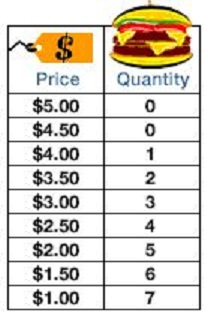
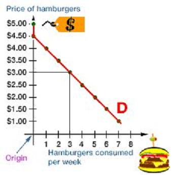
1A.2 [TW 1.2.2
(9:57)] Plotting A Linear Relationship Between Two Variables -
1b
- Outline
- Creating the demand curve
- The demand curve
- Formula for the demand curve
- The slope describes the consumer's behavior when price
changes
- Creating the demand curve
- look at the data and determine the relationship between the
two variables
- draw, LABEL, and calibrate the axes ("calibrate" means put
numbers along the axes)
- the "origin" is the point where the x and y axes
intersect
- plot the data on the graph
- connect the points to draw the demand curve
- The demand curve
- the demand curve shows the relationship between the price
of a good and he quantity a consumer wants to buy
- ME:
- note that as the price of hamburgers goes down then Bob
will buy more hamburgers
- this represents an inverse, or negative,
relationship between price and quantity of hamburgers
purchased
- an downward sloping (from left to right) line on a graph
indicates an inverse relationship
- an downward sloping line will have a negative
slope (we will discuss the idea of slope more
later)
- Formula for the demand curve
- y = a + bx
- y = the vertical axis variable (Price)
- a = the y-intercept
- b = slope
- x = the horizontal axis variable (Quantity)
- in our example:
- Price = $4.50 - $0.50 * Quantity
- P=4.50 -.5Q
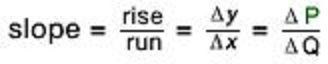
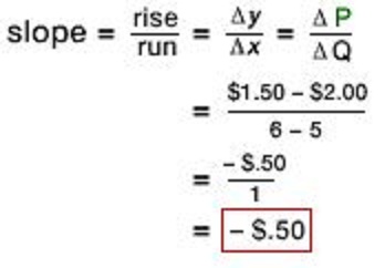
- The slope describes the consumer's behavior when price changes
- b = slope = rise/run =
 y/x
= change in price / change in quantity = P/Q
y/x
= change in price / change in quantity = P/Q
- if the price of hamburgers decrease by $0.50 then Bob will
buy one more hamburger
- b = P/Q
- slope = -$0.50 / 1 = -0.50
- slope is negative indicating the inverse relationship
(or that have to DECREASE the prise to get Bob to
INCREASE the quantity that he will buy)
- ""
means "change"
- ME:
- So, if you know the y-intercept and the
slope of a straight line you can find all of the
possible values for the two variables
- we know that a=4.50 and b=-.50, then
- if the price is $3.00 how many burgers will
Bob buy?
- first, write down the information that you
have:
- price = y = 3.00
- y-intercept = a = 4.50
- slope = b = -.50
- then, write down the formula:
- y = a + bx
- Price = y-intercept + slope times the
quantity
- now, plug the data into the formula
- finally, you can you solve for Q
- subtract 4.50 from each side:
- 3.00 - 4.50 = 4.50 + -50Q - 4.50
- -1.50- = -50 * Q
- then divide each side by -50:
- -1/50/-50 = (-.50Q)/.50
- -1.50/.50 = Q
- 3 = Q;
- if you look at the graph or the table
you can see that we got it right; when the
price was $3.00, Bob bought 3
hamburgers
|
|
1A.3 [TW 1.2.3
(8:42)] Changing the Intercept of a Linear Function - 1b
- Outline
- What happens if we change Bob's income?
- Raising Income
- Lowering income
- Summary
- What happens to the relationship between price and quantity if
we change Bob's income?
- Raising Income
- if Bob gets a higher income we can expect that he will
change his behavior; he will probably buy more hamburgers
- on the demand table we can see that at the same prices, Bob
will buy more hamburgers
- on the graph, with the higher income the y-intercept has
increased and the demand curve has moves to the right
- the slope is still the same so we still have the same
negative relationship, but now with higher quantities
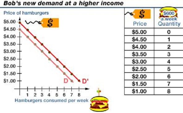
- formula for the new demand if Bob's income increases: P =
5.00 -.50Q
- the curve has shifted to the right
- Lowering income
- we can do the same thing for a lower income causing the
curve to shift to the left
- this will decrease the y-intercept (but keep the slope the
same)
- formula for the demand with a lower income: P = 4.00
-.50Q
- the curve has shifted to the left and the slope stays the
same
- Summary
- a change in income will result in a parallel shift of the
demand curve
1A.4 [TW 1.2.4 (7:28)] Understanding the Slope of a
Linear Function - 1b
- Outline
- What does the slope of a demand curve indicate?
- Units and Slope
- What does the slope of a demand curve indicate?
- the sensitivity of Bob's demand for hamburgers to changes
in the price
- or, what happens to the number of hamburgers that Bob buys
each week when the price changes?
- this will help us understand how economists think about the
slope of a line
-
- in our original example we saw that when the price of
hamburgers fell by $0.50 then Bob would buy one more hamburger
a week
- so if the price goes down from $2.00 to $1.50
- What if the slope of the demand curve changes?; What if Bob
has a different relationship between price and quantity?
- if price = $2.00 then he would buy 5 hamburgers and if
price = $1.50 he would buy 10 hamburgers
- result: and new demand curve with a different slope; a
flatter slope; and smaller slope
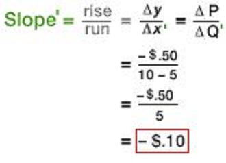
- now Bob is more sensitive to a change in price; now, a
$0.50 decrease in price causes Bob to buy a lot more (5)
hamburgers; or when the price decreases by just a dime
($0.10) he will buy one more hamburger
- the slope of curves indicates the sensitivity of one
variable to changes in another
- Units and Slope
- Warning: the slopes of the curves depends completely upon
the unit in which the variables are measured
- here we were measuring the price of hamburgers in
dollars ($4.00, $3.50, $3.00, etc)
- but the slopes would change if we measured the prices in
cents (400 cents, 350 cents, 300 cents, etc)
- so if we change the way we measure the price, then the
slopes will change
- the same thing happens if we change the way that we
measure burgers (boxes of burger, or half burgers, etc)
- so if we want to measure the sensitivity of one variable to
changes in another we can't use slope since slopes can change
just because we change the units, even though the sensitivity
is the same
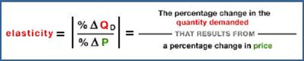
- therefore economists use something class
"elasticity" to measure sensitivity
- the price elasticity of demand is the percentage
change in the quantity demanded that results from a percentage
change in price
- since elasticity uses percentage changes, is doesn't matter
whether we measure the price of hamburgers in dollars or in
cents, the elasticity (sensitivity) will be the same
OPTIONAL: SIMPLE MATH,
ALGEBRA AND GEOMETRY FOR ECONOMICS STUDENTS
How to Multiply and Divide Fractions in Algebra for Dummies
(YouTube fordummies 1:50) - 1b
http://www.youtube.com/watch?v=B7MtFQW7i_I
- 2/5 x 3/7
- 2/3 x 3/8
- 2/3 x 3/7
- 1/3 ÷ 4/5
Simple Equations (11:06) - 1b
http://www.khanacademy.org/math/algebra/solving-linear-equations-and-inequalities/v/simple-equations
- 7x = 14 (very elementary)
- 3x = 15 (6:00 is a good place to start)
- 2y + 4y = 18
Solving One-Step Equations (1:54) - 1b
http://www.khanacademy.org/math/algebra/solving-linear-equations-and-inequalities/v/solving-one-step-equations
- a + 5 = 54; solve for a and check your solution
Solving One-Step Equations 2 (2:23) - 1b
http://www.khanacademy.org/math/algebra/solving-linear-equations-and-inequalities/basic-equation-practice/v/solving-one-step-equations-2
- x/3 = 14; solve for x and check your solution
Solving Ax + B = C (8:41) - 1b
http://www.khanacademy.org/math/algebra/solving-linear-equations-and-inequalities/basic-equation-practice/v/equations-2
- 3x + 5 = 17 (very elementary)
- 7x - 2 = -10 (starting at 5:20)
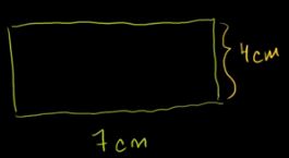
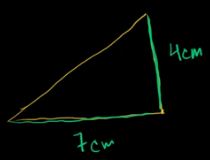
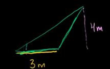
Area and Perimeter (12:20) - 1b
http://www.khanacademy.org/math/geometry/basic-geometry/v/area-and-perimeter
- area of a square
 (very elementary; he does make an adding error!)
- area of a rectangle (begins at 5:00)
- area of a right triangle (begins at 6:44)
- area of a triangle (begins at 10:06)
MODULE 1c - SCARCITY AND BUDGET LINES
- WHAT IS ECONOMICS: SCARCITY, THE 5Es, AND MAKING CHOICES
- 1.1.1 Scarcity - Defining Economics [TW 1.1.1
(6:35)]
- 1.2.1 What Economists Do [TW 1.1.2 (13:20)]
- 1.2.2 Micro and Macroeconomics [TW 1.1.3
(11:21)]
- BUDGET LINES
- 6A-1 Constructing a Consumer's Budget Constraint [TW
3.2.1 (9:36)]
- 6A-2 Understanding a Change in the Budget Constraint
[TW 3.2.2 (5:02)]
1.1.1 [TW 1.1.1 (6:35)] Scarcity - Defining Economics -
1c
- Outline:
- what is economics?
- opportunity costs
- the big picture: economic models
- definition of economics: rational choice under conditions of
scarcity
- what is scarcity?
- ME: limited resources vs. unlimited human wants
- what is rational choice? = self interest, comparing costs and
benefits to maximize satisfaction = calculated self interest
- calculated self interested people operating under conditions
of scarcity = economics
- opportunity cost
- no such thing as a free lunch
- we can make economic models about almost anything
1.2.1 [TW 1.1.2 (13:20)] What Economists Do -
1c
- Outline:
- scientific method
- ask questions
- produce models
- form hypotheses
- where to find economists
- normative vs. positive economics
- the STUDY of economics = social science = uses the scientific
method = asking a question = why?
- what to produce?
- how will it be produced?
- who is going to get what is produced?
- building a scientific model = map = the model (map) that you
use depends on the question being asked providing only the
information needed to answer the question
- hypotheses = predictions on how the world works = can be
tested with data
- building relationships between variables by ignoring variables
that do not matter to the questions being investigated
- ME: models are SIMPLIFICATIONS of reality
- ME add more: GENERALIZATION
- ABSTRACTION
- ask a question
- isolate related variables and build model
- come up with hypotheses that you can test with data
- ceteris paribus: holding all other factors constant to
help see relationships between just two variables
- Positive economics vs normative economics
- positive: what IS happening? what will happen, predictions,
and descriptions how world does work
- normative: what SHOULD we do? judgments What is good? how
world should work
1.2.2 [TW 1.1.3 (11:21)] Microeconomics and
Macroeconomics - 1c
- Outline:
- microeconomics vs. macroeconomics
- players in the economy
- nominal vs. real variables
- microeconomics vs macroeconomics
- individuals vs aggregate, biology analogy: cell vs. whole
organism
- macro: study of the economy as an organism, study of the
overall economy
- micro: how the cell works; individual parts of the
economy
- MICRO: the way a particular household responds to changes in
incentives
- ignores money, relative prices rather than monetary
prices
- MACRO: money is the life blood of the macroeconomic organism
- money carries things through the system,
- difference: individual decision making vs. the whole
organism
- money is more or less ignored in micro vs. money is important
in macro
- the four major players: households, businesses, government,
foreigners (net exports) and how they are studied in micro vs.
macro
- "real" values are measured in terms of physical goods and
services
- "nominal" values are measured in dollar terms, money; $1.25
(nominal) vs a real cup of coffee (real)
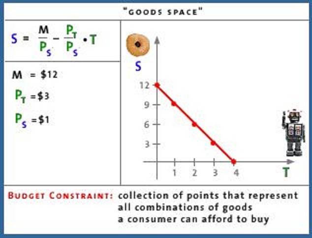
BUDGET LINES
6A-1 [TW 3.2.1
(9:36)] Constructing a Consumer's Budget Constraint - 1c
- Outline
- Consumer dilemma: toys or snacks?
- Plotting points on the budget constraint
- Budget constraint = an equation for a line
- Budget constraint & opportunity cost
- Consumer dilemma: toys or snacks?
- I want it all, but I have a limited amount to spend
- what is feasible (possible) = the budget constraint = what
you can afford
- ME: we are not going to do the indifference curves (or
preferences) and we are not going to derive the demand
curve
- Plotting points on the budget constraint
- vertical axis = quantity of snacks
- horizontal axis = quantity of toys
- The info we need to figure it out
- I only have $ 12 to spend; called your income; income =
$12
- price of toys = $3.00
- price of snacks = $1.00
- What is the maximum number of $1 snacks that you can buy
with your $12? TWELVE
- What is the maximum number of $3 toys that you can buy with
your $12? FOUR
- The video lecture will ask you a
multiple choice question. ANSWER THE QUESTION by selecting A,
B, or C and more of the lecture will follow
- budget constraint (or budget line) shows all
of the combinations of two goods that you can afford to buy
given your limited income and the prices of the goods; it shows
what is feasible or possible
-
- Budget constraint = an equation for a line
- income = (Pt x Qt) + (Ps x Qs); M = Pt*T + Ps*S
- isolate the snack variable because it is on the vertical
axis
- S = M/Ps - (Pt/Ps*T)
- the number of snacks that you can afford EQUALS the number
of snacks that you can afford if you spent your whole income on
snacks MINUS the number of toys that you buy times the relative
price of toys to snacks
- Budget constraint & opportunity cost
- the Pt/Ps term is the opportunity cost of getting another
toy = -3/1 = -3
- so the opportunity cost of getting another toy is that you
have to give up 3 snacks.
- THIS IS WHERE THE VIDEO LECTURE ENDS
The video lecture will ask you a multiple
choice question. BUT there is an error in the video. Just end
the video here
6A-2 [TW 3.2.2 (5:02)] Understanding a Change in the
Budget Constraint - 1c
- Outline:
- Intro
- What can change the budget constraint (budget
line)?
- Effect of a change in income
- Effect of a change in price
- Review: movements of the budget line
- Intro
- the slope of the budget line is Pt/Ps which is the number of
snacks that you have to give up to get one more toy = -3
- What can change the budget constraint (budget line)?
- if your income changes it will change your budget line
- if the prices of the products change it will change your
budget line
- Effect of a change in income -- What happens to the budget
line (what you can afford to buy) if:
- income is reduced
- if income (M) goes from $12 down to $6 then you can
afford to buy LESS
- and the budget line will shift inward but it will
keep the same slope because the relative prices, Pt/Ps, has
not changed
- income is increased
- the budget line will shift outward, but
- keep the same slope because the opportunity cost of toys
measured in terms of snacks (Pt/Ps) has not changed
- Effect of a change in price
- What happens if the price of toys decreases from $3 to
$1.50?
- If your budget is still $12 then you will be able to buy
more toys = 8 toys (8 x $1.50 = $12)
- but you can still buy the same number of snacks
- so the budget line rotates out along the toy
axis
- notice that if the price of toys decreases your budget
line has rotated outwards meaning that you can buy more toys
AND snacks
- Review: movements of the budget line
- if there is a change in income then the budge line SHIFTS,
but the slope stays he same
- if there is a change in price of one of the goods then the
budget line ROTATES and the slope changes
MODULE 1d - PRODUCTION POSSIBILITIES and BENEFIT
COST ANYALYSIS
- PRODUCTION POSSIBILITIES
- 2.1-1 Understanding the Concept of Production Possibilities
Frontiers [TW 1.4.1 24:46)]
- 2.1-2 Understanding How a Change in Technology Affects the
PPF [TW 1.4.2 (10:10]
- 2.1-3 Deriving the Algebraic Equation for the PPF [TW
1.4.3 (21:58)]
- MAKING CHOICES: THE ECONOMIC WAY OF THINKING -- BENEFIT-COST
ANALYSIS (also called Marginal Analysis or Cost-Benefit Analysis)
2.1-1 [TW 1.4.1 24:46)] Understanding the Concept of
Production Possibilities Frontiers - 1d
- Outline:
- scarcity and efficiency
- production possibilities table
- production possibilities curve
- calculating opportunity costs
- production possibilities curve - PPC (also called the
production possibilities frontier - PPF) and scarcity
- first: discuss efficiency: doing the best with what you have =
getting the most you can from what you have
- efficient behavior is to produce the most wheat with a given
quantity of rice
- only two goods produced - what is the optimal output of wheat
and rice this economy can produce
- need to know what resources and what technology is
available
- ME: our textbook lists 5 assumptions of the production
possibilities curve:
- fixed resources
- fixed technology
- productive efficiency
- full employment
- only two goods being produced
- technique vs. technology
- technique = a particular combination of inputs
- technology = all the possible combination of inputs = a
catalog of all the things an economy knows how to do
- improved technology = more output with less input
- production possibilities table : every combination is an
"efficient" combination that can be produced = maximum amount that
can be produced
- ME: Note how Professor Tomlinson is moving the "best suited"
resources first to the production of rice; this allows a large
increase of rice production with only a small loss of wheat
production
- "efficient combination of resources" means that we are
producing the maximum quantities possible
- the production possibilities curve (PPC) is also called the
production possibilities frontier (PPF)
- first label the axes
- then calibrate the axes
- now plot the points that represent the possible combinations
of wheat and rice that can be produced
- ME: any point on a graph represents two numbers; don't get
scared, all we are doing is looking at only TWO NUMBERS for each
point on the graph
- then connect the dots to draw the graph
- NOTE: the shape of the PPC
- PPC is a collection of points representing the maximum
combinations of output an economy can produce given that economy's
technology and resource endowment (amounts)
- What the PPC represents:
- points (quantities of wheat and rice) outside of the curve
are not attainable (ME: such quantities are IMPOSSIBLE
with the given technology and resources THEREFORE WE MUST
MAKE CHOICES)
- points within the PPC are possible but are less than the
maximum possible. If there is inefficiency or unemployment then
less than the maximum possible will be produced and the economy
will be at a point within their PPC
- a point within the curve (i.e. less output) is also what
happens if there are UNEMPLOYED resources
- ME: when Tomlinson is discussing using wet land for
wheat and dry land for rice he is talking about
PRODUCTIVE INEFFICIENCY - not using resources
where they are best suited (from the online 5Es lecture). He
calls this the "underemployment of resources". I call this
"productive inefficiency" (5Es)
- OPPORTUNITY COST = downward sloping PPC; wheat is
the opportunity cost of rice: Why?
- CALCULATING THE OPPORTUNITY COST. Know how to do
this!
- opportunity cost = change in wheat/change in rice
- opportunity cost is the slope of the line connecting the
two points
- Why does the opportunity cost (slope) of producing rice
increase as more rice is produced?
- i.e. why does the PPC get steeper as we increase the
quantity of rice?
- shape of PPC is CONCAVE (bowed out)
- ME: our textbook calls this the "Law of Increasing
Costs"
- WHY?
- Because not all resources are the same. Some are
better for producing rice and others are better suited to
producing wheat
- this causes the opportunity costs to increase as we
produce more rice
- i.e. this causes the shape of the PPC to be concave
(bowed out)
- SUMMARY: 4 things we can see in the PPC
- some combinations are impossible so therefore there is
scarcity AND we must then make choices
- unemployed resources and productive inefficiency causes
less than the maximum level of production
- there are opportunity costs
- the PPC is concave representing increasing opportunity
costs because not all resources are the same, some are better
suited to producing rice and others are better suited to
producing wheat
2.2-2 [TW 1.4.2 (10:10)] Understanding How a Change in
Technology or Resources Affects the PPC - 1d
- Outline:
- production possibilities curve
- outward shift (ME: called "economic growth")
- individual product shift
- inward shift
- summary
- What happens if there is a change in technology or amount of
resources? PPC will shift out
- What is the difference between an movement along an existing
PPC and shifting the curve to a new curve?
- If BETTER TECHNOLOGY for rice and wheat production is
discovered, the curve will shift outward representing that MORE
can be produced i.e the quantities on the production possibilities
table get larger
- What if we get MORE RESOURCES like more labor? Answer: PPC
shifts outward
- ME: our textbook calls this "economic growth".; Definition:
and increase in the ABILITY to produce caused by getting more
resources, getting better resources, or getting better
technology
- What if we ONLY get better technology for wheat but not for
rice? A "skewed" shift outward of the PPC.
- What if there is a change in climate hurting the production of
wheat but helping the production of rice? Again, a "skewed" shift
outward of the PPC.
- What if there are FEWER RESOURCES? The PPC will shift
inwards
- ME: there is a big difference between moving from a point on
the curve to moving to a point inside the curve AND the whole
curve shifting inward
- moving from a point on the curve to to a point inside the
curve is caused by not using all available resources
(unemployment) or productive inefficiency. If this happens we
still CAN produce the same quantities as before, but we are
just not achieving our potential; our possible production did
not change
- the whole curve shifting inward is caused by there being
fewer resources than before (depletion) and now the maximum
that can be produced is less; out potential has decreased
- QUESTION: Which combination of wheat or rice is
preferred? ME: Which is the allocatively efficient quantity?
ANSWER:"We have no idea." The PPC is not designed to tell us what
we want. It is designed to tell us what is possible. We will have
a different model in a later chapter to tell us what we want -
what quantities will maximize our satisfaction (allocative
efficiency)
- ME: when Tomlinson is discussing "efficiency" he seems
to be discussing only PRODUCTIVE EFFICIENCY. Now would be a good
time to re-read the 5Es lecture: http://www.harpercollege.edu/mhealy/eco212i/lectures/ch1-18.htm
2.1-3 [TW 1.4.3 (21:58)] Deriving the Algebraic
Equation for the Production Possibilities Frontier - 1d
- Outline
- unit labor requirement
- production possibilities schedule
- production possibilities graph
- formula for the production possibilities line
- significance of the line
- Another view of the PPC, good review
- ME: why is Bernie's PPC a straight line? NOT CONCAVE
- ME: You do NOT have to know the algebraic
equation
- A straight line can be described with an algebraic
equation: y = mx + b
- y = vertical axis variable = SW
- m = slope
- b = vertical intercept = 6
- x = horizontal axis variable = SC
- SW = 2SC + 6 or y = 2x + 6
MAKING CHOICES: THE ECONOMIC
WAY OF THINKING -- BENEFIT-COST ANALYSIS (also called Marginal
Analysis or Cost-Benefit Analysis)
Thinking at the Margin (LearnLiberty 4:32) - 1d
http://www.youtube.com/watch?v=tMhdTn-5fu8
- ME: "marginal" means "extra" or "additional"
- individuals make choices based on comparisons at the
margin
- when wanting to make the best choice we compare the
options
- "thinking at the margin" means we look at the next option
- why are diamonds more expensive than water?
- because when you compare the value of an extra unit of
water (the marginal unit) with the extra unit of diamonds
- we make choices at the margin all the time, also businesses
- should we hire an extra employee
- we compare the extra cost of that employee, called the
marginal cost (MC)
- with the extra benefits that we will get from that worker
-- i.e. the marginal benefit (MB)
Incentives and Marginal Analysis (MrHurdleHistory 8:54) -
1d
http://www.youtube.com/watch?v=dN9KyDCur2Y
- to make the best decision:
- select all options where the MB > MC
- up to where the MB = MC
- but never where the MB < MC
- the BEST CHOICE is always where MB =MC
- changes in MB and MC:
- if the MB increase, people will do more
- if the MB decrease then people will do less
- if the MC increase then people will do less
- if the MC decrease then people will do more
Chapter 2 (Module 2a)
MODULE 2a - MARKET ECONOMIES AND TRADE
- ECONOMIC SYSTEMS
- SPECIALIZATION AND GAINS FROM TRADE
- 2.2-1 Defining Comparative Advantage with the PPF [TW
1.5.1 (22:40)]
- 2.2-2 Understanding Why Specialization Increases Total
Output [TW 1.5.2 (6:46)]
- 2.2-3 Analyzing International Trade Using Comparative
Advantage [TW 1.5.3 (25:35)]
ECONOMIC SYSTEMS
[TW 1.1.4 (10:50)] An Overview of Economic Systems -
2a
$1.98 at http://mindbites.com/lesson/7393-economics-an-overview-of-economic-systems
- Outline
- Three Economic Questions
- Pure Laissez-faire economic system
- Centrally-planned economic system
- Mixed economic systems
- Every economic system must answer three questions
- What will be produced
- How will it be produced
- Who will get what is produced
- ME: the textbook lists five fundamental questions
- What goods and services will be produced?
- How will the goods and services be produced?
- Who will get the goods and services?
- How will the system accommodate change?
- How will the system promote progress?
- Pure Laissez-faire economic system - One EXTREME
- "Laissez-faire" is French for "leave us alone" or "let us
do"
- everyone makes their own decisions
- prices arise in a market and these prices provide
incentives to guide resources
- the role of prices is very important in coordinating the
use of resources
- law of the jungle
- maximum individual freedom
- all people respond according to what they perceive is best
for them
- problems:
- end result might end up not being best fit society as a
whole
- examples of when the end result may be bad: (1)
standing up at a football game, (2) litter, (3) when
prices are not available to guide decisions like for
clean air
- monopolies may form
- Centrally Planned Economy - the other EXTREME
- central idea: a wise central planner make all the decisions
of when recourses would be used and how to generate wealth for
society
- Problems - where does the central planner get the
information to make good decision and how do they get each
resource to do what is assigned
- via less freedom or monetary incentives?
- central planner does not have all the information
needed
- how do you keep the central planner from abusing their
power and work for the best interest of the society rather
than do what is best for themselves?
- Show which extreme view is better?
- In the real world all economic systems are MIXED
SYSTEMS including parts of laissez faire and part of central
planning
- US: mostly laissez-faire with some central planning
- China: a lot of central planning and some
laissez-faire
- The role of the government in these mixed systems then is to
regulate the mix of these two extremes, some allow more
laissez-faire and some do more central planning
- a spectrum or continuum of mixed economic systems
Power of the Market (LibertyPen 1:14) - 2a
http://www.youtube.com/watch?v=4FHxpoQqPTU
- Milton Friedman (July 31, 1912 November 16, 2006) was an
American economist, statistician, and author who taught at the
University of Chicago for more than three decades. He was a
recipient of the Nobel Prize in Economics
- the invisible hand of capitalism -- what is it?
[TW 17.5.3 (12:16)] Comparative Economic Performance -
2a
$1.98 at: http://www.mindbites.com/lesson/7658-economics-comparative-economic-performance
- Outline
- The Bolshevik Revolution
- Contributing factors to the collapse of the Soviet
Union
- Movement back to free-market economy
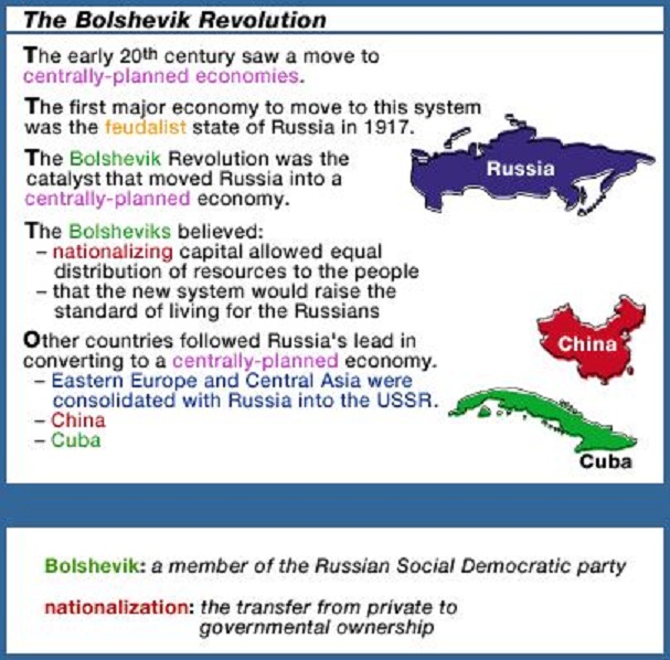
- The Bolshevik Revolution
- Forced the movement from a decentralized economy
to a centrally planned economy in Russia in the early
20th century
- they nationalized capital -- the government
took over businesses
- goal was to increase the standard of
living
- With no motivational incentives to produce high
quality goods, production slowed considerably
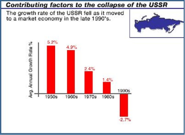
- in the 1950s and 60s the economy of the Soviet
union grew at a grate of 5%-6% -- about the same or
faster than other countries with market
economies
- 1970s this rate slowed to about 2-3%, 1980s
1-2%, 1990s recession
- Why?
|
|
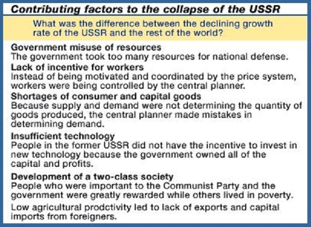
- Contributing factors to the collapse of the Soviet Union
- government took too many resources -- 15% of GDP
used for national defense vs. 6% in the US
- lack of incentives for workers ;ME: the incentive
problem from the textbook
- misallocation of resources caused shortages; ME:
the coordination problem from the textbook
- Soviet technology was a decade behind because
there was no profit motive to encourage investment in
new technology
- A two-class society developed
- ME: see the textbook for
- the incentive problem
- the coordination problem
|
|
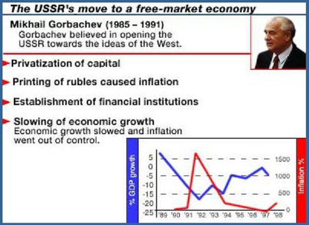
- Movement back to free-market economy
- In the late 1980s, through Mikhail Gorbachev's
ideals of glasnost and perestroika, the
Soviet Union began its transformation in response to
the failed planned economy
- Resources were privatized
- ownership would serve as an incentive to
achieve efficiency
- Government printed rubles (money) causing
inflation
- prices of goods and services were deregulated and
allowed to be set by supply and demand
- Russia did not have the financial institutions
that established free market economies did; little
protection of property rights
- organized crime rose in the early 1990s ; a mafia
arose
- Economic growth slowed
|
|
- Summary
- The Czech republic soon attained 5% growth while Russia
didn't
- Capitalism is a success and Communism is a failure?
- too simplistic of a conclusion
- we have some central planning in the US - a mixed
economy
- but the Russian experiment did fail as compared to
similar market economies
SPECIALIZATION AND GAINS FROM TRADE
2.2-1 [TW 1.5.1 (22:40)] Defining Comparative Advantage
with the Production Possibilities Curve - 2a
- Outline
- Anne's Production Possibilities
- Comparing Production Possibilities curves
- Specializing and Trading
- Creating More Output
- Anne's Production Possibilities
- ME:
- The concept of comparative advantage can be used to show
how two people (or two countries) with different abilities
(or resources) can cooperate (or trade) to increase their
wealth
- we will show how countries gain from international
trade
- we will be using straight line production possibilities
curves for two different people (Bernie [previous
lecture] and Anne) to show how together they can do more
than if they cooperate (trade)
- Note that Anne can BOTH scrub and sweep more than can
Bernie; we say that Anne has an absolute advantage in
doing both tasks since she can do them with fewer resources;
i.e. Anne is better at doing both
- Anne's production possibilities schedule shows the various
maximum combinations of sweeping and scrubbing maximum number
of rooms that she can do in one hour
- Comparing Production Possibilities curves: finding the
opportunity costs
- Calculate Anne's opportunity costs of sweeping and
scrubbing"
- 1 room swept = 1 room not scrubbed
- 1 room scrubbed = 1 room not swept
- Calculate Bernie's opportunity costs
- 1 room swept = 1/2 room not scrubbed
- 1 room scrubbed = 2 room not swept
- a straight line PPC means that the opportunity costs are
constant; for a country it would mean that we would assume a
that all resources within that country are the same; remember
in a previous lecture we said that a PPC is usually concave to
the origin (bowed out) because not all resources are the
same. Some are better for producing one product and others are
better suited to producing something else
- this causes the opportunity costs to increase as we
produce more of one product
- i.e. this causes the shape of the PPC to be concave
(bowed out)
- BUT when discussing comparative advantage we usually assume
that all resources within a country are the same so that we get
constant opportunity costs and a straight line PPC: this makes
our work easier
- Specializing and Trading
- Here are the opportunity costs again:
- Anne's opportunity costs of sweeping and
scrubbing
- 1 room swept = 1 room not scrubbed
- 1 room scrubbed = 1 room not swept
- Bernie's opportunity costs
- 1 room swept = 1/2 room not scrubbed
- 1 room scrubbed = 2 room not swept
- What if they worked independently:
- then they can only sweep and scrub a number of rooms
that is on their PPC
- lets ASSUME that Bernie sweeps 2 rooms and scrubs 2
rooms
- lets ASSUME that Anne sweeps 6 rooms and scrubs 6
rooms
- they of course could clean different combinations, but
let's just use this as our given starting point
- Creating More Output
- working independently, what are the total number of rooms
that are swept and scrubbed?
- scrubbing: Bernie 2 rooms + Anne 6 rooms = 8 rooms
scrubbed
- sweeping: Bernie 2 rooms + Anne 6 rooms = 8 rooms
swept
- remember this is one of the MAXIMUM combinations
possible if they work independently
- But what if they specialize according to their
comparative advantages? Then, how many rooms can be scrubbed
and swept?
- a person has a comparative advantage at an activity
if they can perform that activity at a lower opportunity cost
than anyone else; i.e. if they give up less than other
people when they do the activity
- We will show that if Bernie and Anne specialize according
to their comparative advantages that they can scrub and sweep
MORE ROOMS THAN IF THEY WORKED INDEPENDENTLY
- who has a comparative advantage in scrubbing? --
that is, who has a lower op cost of scrubbing OR who gives
up sweeping fewer rooms when they scrub
- ANNE: 1 room scrubbed = 1 room not swept
- Bernie: 1 room scrubbed = 2 room not swept
- Anne has a lower op cost of scrubbing = 1room
not swept; if she scrubs a room she gives up fewer rooms
not swept -- just 1) whereas If Bernie scrubbed a room he
would give up 2 rooms not swept.
- so Anne has a comparative advantage in
scrubbing and she should specialize in scrubbing
- who has a comparative advantage in sweeping? --
that is who has a lower op cost of sweeping OR who gives up
scrubbing fewer rooms when they sweep
- ANNE: 1 room swept = 1 room not scrubbed
- Bernie: 1 room swept = 1/2 room not scrubbed
- Bernie has a lower op cost of sweeping = 1/2 room not
scrubbed; if he sweeps a room he gives up fewer rooms not
scrubbed -- just 1/2) whereas If Anne swept a room she
would give up 1 rooms not scrubbed.
- so Bernie has a comparative advantage in sweeping
and he should specialize in sweeping
- People, or countries, should specialize in (do more of)
those things in which they have a comparative advantage; in
which they give up the least. When they do this MORE will
be produced
- We will see how in the next lecture
2.2-2 [TW 1.5.2
(6:46)] Understanding Why Specialization Increases Total Output -
2a
- Outline
- Bernie and Anne Continued
- Recognizing specialization
- Conclusion
- Bernie and Anne Continued
- Bernie has a comparative advantage in sweeping and he
should specialize in sweeping
- Anne has a comparative advantage in scrubbing and she
should specialize in scrubbing
- So lets have Bernie ONLY SWEEPS and in one hour he will be
able to sweep 6 rooms (and scrubbing 0)
- And, let's have Anne do more scrubbing, let's say she
scrubs 9 rooms. leaving her time to sweep 3 rooms
- What happened to total number of rooms scrubbed and swept?
- by specializing according to their comparative
advantages together they are now sweeping 9 rooms (6 by
Bernie and 3 by Anne) and scrubbing 9 rooms (all by
Anne)
- REMEMBER: in the previous lecture we said that working
independently they could only sweep and scrub 8 rooms, BUT by
specializing and trading they can now sweep ands scrub 9 rooms,
in the same amount of time
- ME: with the same amount of resources (one hour of work
each), by specializing according to their comparative
advantages, MORE ROOMS were swept and scrubbed! EVEN THOUGH
Anne is better at doing both.
- Recognizing specialization
- Conclusion
- the trader with the flatter PPC will have a comparative
advantage for providing the good or service on the horizontal
axis (assuming the graphs are calibrated the same)
- if you have a comparative advantage in one good then you
have a comparative disadvantage for the other good
- everyone has a comparative advantage in something
- by specializing according to comparative advantage
everyone who is trading can gain!
2.2-3 [TW 1.5.3 (25:35)] Analyzing International Trade
Using Comparative Advantage (over 20 minutes) - 2a
- Outline
- Constraints of Two Countries
- Graphing Production Possibilities
- Benefits of Trading
- Constraints of Two Countries
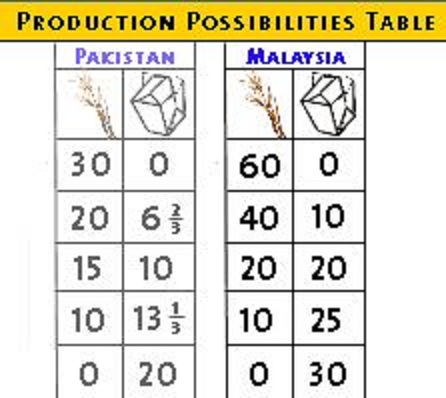
- Pakistan's unit labor requirement: the amount of time it
takes to perform a task
- 1 wheat takes 2 workers
- 1 rice takes 3 workers
- now we can calculate the opportunity cost
- 1W = 2/3 R
- 1R = 3/2 W = 1 1/2 W
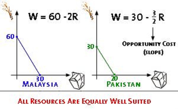
- if Pakistan has only 60 workers then it can produce
- a maximum of 30 W
- OR a maximum of 20 R
- now we can draw the PPC for Pakistan
- Malaysia with a different technology can produce
- 1 W with 1 worker, and
- 1 R with 2 workers
- Malaysia has an absolute advantage in producing both
wheat and rice; i.e. they are better at producing both
- now we can calculate the opportunity costs in Malaysia
- 1 W= 1/2 R; every time they produce a bushel of wheat
it takes them 1 worker who could have produced 1/2 bushel
of rice
- 1 R = 2 W
- if Malaysia has only 60 workers then it can produce
- a maximum of 60 W
- OR a maximum of 30 R
- now we can draw the PPC for Malaysia
- Graphing Production Possibilities
- PPC is a straight line
- which means the opportunity cost is constant; it means we
are assuming all of the recourses in Pakistan are the same and
all of the resources in Malaysia are the same;
- if some resources in one country were better at producing
wheat and some were better at producing rice then the PPC would
be concave (bowed out) and we would have increasing costs
- we could have also plotted the PPC using the equation for a
straight line
- opportunity costs again and now we can see which country has a
comparative advantage in which product:
- Benefits of Trading: Showing how both countries can gain from
specialization and trade
- you will be given an initial starting point when countries
are not trading; when they are independent of each
other; one of the points along their PPC
- Malaysia: 20 R and 20 W
- Pakistan: 10 R and 15 W
- total production when acting independently: 30 R and 35
W
- how can they gain if they specialize according to their
comparative advantage and trade?
- opportunity costs again and now we can see which country
has a comparative advantage in which product:
- find comparative advantage:
- Pakistan because its op cost of rice (3/2) is lower
than the op cost of rice in Malaysia (2 W); so Pakistan
has a comparative advantage in rice and it should produce
more rice
- Malaysia has a comparative advantage in wheat (2/3 is
less than 2); so Malaysia should produce more wheat
- Gains from trade:
- IF Pakistan produces ONLY RICE it can produce
20R
- if Malaysia produces 12 R it can still produce 36
W
- totals with trade: 32R and 36 W
- total (from above) without trade: 30 R and 35 W
- GAINS from trade: 2 more R and 1 more W have been
produced with the same amount of resources
- ME: our textbook discusses 100% specialization
meaning the Pakistan only produces rice and Malaysia only
produces wheat. Lets see how both countrys can gain from trade:
- assume BEFORE they specialize:
- Pakistan produces15W and 10 R, and
- Malaysia produces: 40 W and 10 R
- Total BEFORE specialization: 55W and 20 R
- now if both countries only produce the products in which
they have a comparative advantage (100% specialization)
- Pakistan produces 20R, and
- Malaysia produces: 60W
- Total AFTER specialization: 60W and 20 R
- Gains from specialization and trade (compare BEFORE
with AFTER): 5 more W are bing produced from the same
amount of resources.
Chapter 3 - Supply and Demand (Modules 3a, 3b, and
3c)
MODULE 3a - DEMAND
- 3.1-1 Understanding the Determinants of Demand Demand [TW
2.1.1 (11:58)]
- 3.1.2 Understanding the Basics of Demand [TW 2.1.2
(11:54)]
- 3.1.3 Analyzing Shifts in the Demand Curve [TW 2.1.3
(8:13)]
- 3.1-4 Changing Other Demand Variables [TW 2.1.4
(10:43)]
- 3.1-5 Deriving a Market Demand Curve [TW 2.1.5
(9:16)]
- OPTIONAL
3.1-1 [TW 2.1.1 (11:58)] Understanding the Determinants
of Demand - 3a
- Outline:
- The determinants of demand
- Building the demand function
- The determinants of demand
- The determinants of demand
- Building the demand function
- The determinants of demand
- ME: In chapter 3 of our textbook the authors list five
"non-price determinants" of demand, but in the video lecture
there are really only 4 non-price determinants of demand. Our
textbook adds: THE NUMBER OF POTENTIAL CONSUMERS that is not in
the video lecture.
- Textbook's non-price determinants of demand: Pe, Pog, I,
Npot, T
- Pe = expected price
- Pog = price of other goods including the price of
complements and the price of substitutes
- I = income
- Npot = the number of potential consumers
- T = tastes and preferences
Video lecture's non-price determinants of demand: Pc, Ps,
M, Ta, Ex
- Pc = price of complementary goods (Pog in the
textbook)
- Ps = price of substitute goods (also Pog in the
textbook)
- M = income (I in the textbook)
- Ta = tastes and preferences (T in the textbook)
- Ex = expected price (Pe in the textbook)
- we will be building a model of the market
- the market is a place where buyers and sellers
trade some good or service determining the price of the
product and the quantity sold; interaction between buyers
and sellers
- demand is the quantity of a good or service that
households want and are able to purchase in a given time
period
- ME: our textbook defines demand as a schedule
that shows the various quantities of a good or
services that consumers are willing and able to buy at
various prices in a given time period, ceteris
paribus
- supply is the quantity of a good or service that
firms want ands are able to sell in a given time period
- ME: ME: our textbook defines supply as a
schedule that shows the various quantities
of a good or services that businesses are willing and
able to sell at various prices in a given time
period, ceteris paribus
- equilibrium is the market condition in which the
interaction f buyers and sellers finds a particular price
and quantity to be traded and from which there is no
incentive to move
- demand describes the behavior of households
- what are the factors (determinants) that influence how much
of a product (bread) consumers will buy?
- the price of bread
- the price of complementary goods (cheese or
bologna)
- the price of substitute goods (bagels)
- income
- tastes and preferences
- expectations of what might happen to the price of bread
in the future
- ceteris paribus assumption: all other factors
are held constant
- the price of bread
- Law of Demand: as the price of a good or service
increases, the quantity purchased generally decreases,
ceteris paribus; there is an inverse relationship
between the price of bread and the quantity demanded
- Why?
- income effect: there is a decrease in
purchasing power when the price of bread
increases
- substitution effect: when the price of
bread increases people will substitute other products
in place of bread and buy less bread
- ME: our textbook adds a third explanation for the
law of demand: diminishing marginal utility --
as we consume more bread we get less extra
satisfaction from each additional piece (i.e. we start
to get sick of it) and therefore we will not buy more
unless the price is lower since we are getting less
satisfaction
- the price of complementary goods (cheese or bologna)
- complementary goods are two goods for which:
- a decrease in the price of one leads to an increase
in the demand for the other, or
- an increase in the price of one leads to a decrease
in demand for the other
- they are goods that are used together like butter or
cheese or bologna that are used along with bread
- so if the price of peanut butter goes up a person will
probably make fewer peanut butter sandwiches and therefor
the demand for bread will go down
- the price of substitute goods (bagels)
- substitute goods are two goods for which
- an increase in the price of one good leads to an
increase in the demand for the other, or
- a decrease in the price of one leads to a decrease in
demand for the other
- so if the price of bagels goes up some people will
switch to bread increasing the demand for bread
- or if the price of bagels falls some people will buy
more bagels instead of bread which will decrease the demand
for bread
- ME: Tomlinson does make a few errors in how he uses the
terms "demand" and "quantity demanded", but he will discuss
and compare these concepts in a later lecture
- income
- normal goods are goods where if your income increases
then the demand for that good will increase
- if you have more money you will buy more normal
goods
- an inferior good is one where if your income increases
demand for the good will decrease
- if you have more money you will buy fewer inferior
goods
- examples: public transportation, potted meat,
beans,
- tastes and preferences
- if people decide that they now like bread better than
they did before then the demand for bread will increase
- ME: the tastes and preferences determinant is often used
for everything else that may influence the demand for a good
or service
- expectations of what might happen to the price of bread in
the future
- if you think that the price will go up in the future
then the demand for bread will go up now
- Building the demand function
- a mathematical expression that shows how the quantity of
bread that household will purchases is a function of these
variables
- Qd = D(Px, Pc, Ps, M, Ta, Ex)
- ME: if we used the determinants and abbreviations from the
textbook then the demand function will look like this: Qd=D(Pe,
Pog, I, Npot, T) or P, P, I, N, T
- NEXT: we will focus our attention on the PRICE of the product
itself and assume that all of the other variables are held
constant, or do not change, this way we will construct the demand
curve
- ME: For MY explanation of the demand and supply determinants
see: http://www.harpercollege.edu/mhealy/eco212i/lectures/ch3-18.htm
3.1.2 [TW 2.1.2
(11:54)] Understanding the Basics of Demand - 3a
- Outline:
- The demand function
- The demand curve
- The law of demand
- Rationales behind the law of demand
- The demand function
- a mathematical relationship that predicts the quantity of a
good demanded as a function of each of the factors that
influence consumer behavior
- Qd = D(Px, Pc, Ps, M, Ta, Ex)
- ME: if we used the determinants and abbreviations from the
textbook then the demand function will look like this: Qd=D(Pe,
Pog, I, Npot, T) or P, P, I, N, T
- we will focus our attention on the PRICE of the product
itself, ceteris paribus (assuming that all of the other
variables are held constant, or do not change) this way we will
construct the demand curve
- The demand curve
- the graphical relationship between the price of a good and
the quantity demanded, ceteris paribus
- the demand schedule:
- a set of data showing the relationship between price and
quantity demanded, ceteris paribus
- for each possible price of bread there is a quantity
that households will buy in a week, ceteris
paribus
- always label the axes when you draw a graph in economics
- price on the vertical axis and quantity purchased per
week on the horizontal axis
- plot the data from the demand schedule
- note that there are many more prices and many more
quantities that those that we have on our demand schedule so
therefore we can connect the dots on our graph with a smooth
line which is the demand curve
- The law of demand
- the demand curve is downward sloping which shows the law of
demand
- there is an inverse relationship between price and quantity
demanded
- as the price of a good increases, consumers are willing
and able to buy less of it
- as the price of a good decreases, consumers are willing
and able to buy more of it
- note that there are a few exceptions, but in general the
law of demand
- Rationales behind the law of demand -- they explain why the
law of demand is true and why the demand curve is downward sloping
- substitution effect: when the price of bread
increases people will substitute other products in place of
bread and buy less bread
- income effect: there is a decrease in purchasing
power when the price of bread increases
- ME: our textbook adds a third explanation for the law of
demand: diminishing marginal utility -- as we consume
more bread we get less extra satisfaction from each additional
piece (i.e. we start to get sick of it) and therefore we will
not buy more unless the price is lower since we are getting
less satisfaction
3.1.3 [TW 2.1.3
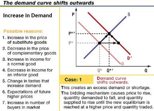
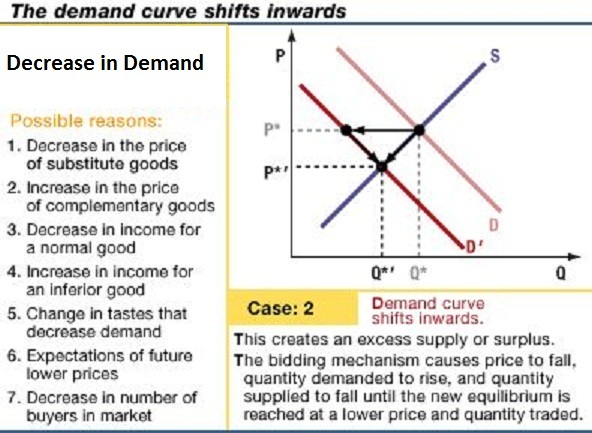
(8:13)] Analyzing Shifts in the Demand Curve - 3a
- Shifting the demand curve
- Assuming bread is a normal good, if there is an increase in
household income, what will happen to the demand for bread?
- what will happens to the quantity demanded at each
possible price?
- note: we are keeping the other non-price determinants of
demand constant (ceteris paribus)
- we get a NEW demand schedule so there has been an increase
in demand
- there will be a larger quantity of bread "at every
price"
- on the graph it looks like the demand has shifted to the
LEFT
- ME: note the direction of the arrows. The demand
shifts to the left (horizontally), it does not shift
up and to the right.
- A "Change in Quantity Demanded" vs."Change in Demand"
- this is very important
- they are not the same thing
- a change in quantity demanded is caused by a
change in the price and it is a movement along a single
demand curve
- a change in demand is caused by a change in one of the
non-price determinants of demand (not price) and it results
in a whole new demand curve either to the right
(increase in demand) or to the left (decrease in demand) of
the original demand curve.
- we have a new demand schedule
- we have a new demand curve
- therefore we have a change in demand
- ME: You need to know the difference between a "change in
quantity demanded" and a "change in demand". THEY ARE
NOT THE SAME THING!
- I often ask students in my face-to-face courses "if the
price of pizza increases, what happens to the demand for
pizza?" The correct answer is NOTHING HAPPENS TO THE
DEMAND FOR PIZZA IF THE PRICE OF PIZZA GOES UP.
- If the price of a product changes then there is a
"change in quantity demanded". On the graph you would
move from one point to another point along the SAME DEMAND
CURVE. The demand curve did not change, just the quantity
demanded changed
- In this video lecture we we discussed a "change in
demand" itself, i.e. creating a whole new demand schedule
and demand curve. When there is a change in demand you get a
new demand curve, or the demand curve will shift to to a new
position. This is NOT caused by a change in the price of a
product, but it IS caused by a change in the "non-price
determinants of demand" (Pe, Pog, I, Npot, T) that we held
constant when we developed the demand concept.
3.1-4 [TW 2.1.4
(10:43)] Changing Other Demand Variables - 3a
- Outline:
- Factors that influence consumer demand
- Variables that shift the demand curve
- Factors that influence consumer demand
- a change in the quantity demanded
- P
 causes Qd
- P
causes Qd
- If the price of a product changes then there is a
"change in quantity demanded"
- the graph does not shift (there has been no change in
demand)
- a change in demand
- a change in one of the non-price determinants of demand
that previously were held constant will cause a change in
demand: a whole new demand curve
- Variables that shift the demand curve
- Video lecture's non-price determinants of demand: Pc, Ps,
M, Ta, Ex
- Pc = price of complementary goods (Pog in the
textbook)
- Ps = price of substitute goods (also Pog in the
textbook)
- M = income (I in the textbook)
- Ta = tastes and preferences (T in the textbook)
- Ex = expected price (Pe in the textbook)
- Textbook's non-price determinants of demand: Pe, Pog, I,
Npot, T
- Pe = expected price
- Pog = price of other goods including the price of
complements and the price of substitutes
- I = income
- Npot = the number of potential consumers
- T = tastes and preferences
- change in the price of other goods -- substitutes
- if there is an increase in the price of bagels, this
will cause an increase in demand for bread (shift to the
right)
- if there is a decrease in price of a substitute good
(bagels), there will be a decrease in demand for the
original product (bread)
- change in the price of other goods -- complementary goods
- if there is an increase in the price of cheese, this
will cause a decrease in demand for bread (shift to the
left)
- if there is a decrease in price of a substitute good
(cheese income), there will be an increase in demand for the
original product (bread)
- change in incomes and normal goods
-
- definition: a normal good is one where demand increase
if income increase
- if incomes increase the demand for normal goods will
increase (shift to the right)
- if incomes decrease the demand for normal goods will
decreases
- change in incomes and inferior goods
- definition: an inferior good is one where demand will
decrease if incomes increase
- Examples: beans, used clothing, potatoes, public
transportation, rice, ramen noodles
- ME: note: a normal good for someone might be a normal
good for someone else
- ME: finally -- "inferior" does not mean "lower quality";
all it means is we will buy less if our incomes increase and
more if our incomes decrease
- if incomes increase the demand for inferior goods will
decrease
- if incomes decrease the demand for inferior goods will
increase
- ME: change in tastes and preferences
- if preferences change in favor of a product then demand
will go up (shift to the right)
- if preferences turn away form a product then demand will
go down (shift to the left)
- change in expected price
- if you expect the price to go up in the future then
demand today will go up (shift to the right)
- if you expect the price to down in the future than
demand today will go down (shift to the left)
- ME: change in the number of potential consumers (see the
textbook)
- if the number of potential consumers increases then
demand for the product will increase (shift to the
right)
- if the number of potential consumers decreases the the
demand for the product will decrease (shift to the
left)
- Summary -- KNOW THIS !!!
3.1-5 [TW 2.1.5
(9:16)] Deriving a Market Demand Curve - 3a
- Outline:
- Recall the Demand Function
- The Market Demand Curve
- Recall the Demand Function
- we have been discussing an individual household's demand
for bread
- now we will look at demand for bread in the whole market
where there are many households each with different individual
demand curves
- The Market Demand Curve
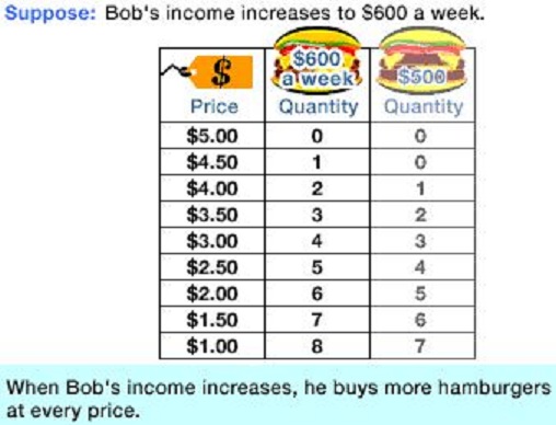
- let's assume that there are only two people in the market:
Bob and Ann
- in order to find the market demand we add together the
individual demand schedules; that is at each price we
add the quantities of all the individuals in the market
- graphically the market demand is the horizontal
summation of all individual demand curves in the market
- quantity is on the horizontal axis so when we add the
quantities of all individuals the result is the market demand
is the horizontal summation of all individual demand curves in
the market
- for any price we add the quantity (horizontal distance to
the demand curve) of all people in the market to get the market
demand curve
- anything that shifts the individual demand curves will
shift the market demand curve; the non-price determinants of
demand (Pe, Pog, I, Npot, T) will shift the market demand
curve
MODULE
3b - SUPPLY
- 3.2-1 Understanding the Determinants of Supply [TW 2.2.1
(6:00)]
- 3.2-2 Deriving a Supply Curve [TW 2.2.2 (9:49)]
- 3.2-3 Understanding a change in Supply versus a Change in
Quantity Supplied [TW 2.2.3 (6:52)]
- 3.2-4 Analyzing changes in Other Supply Variables [TW
2.2.4 8:47)]
- 3.2-5 Deriving a Market Supply Curve from Individual Supply
Curves [TW 2.2.5 (7:16)]
3.2-1 [TW 2.2.1
(6:00)] Understanding the Determinants of Supply - 3b
- Outline:
- The role of profits
- The determinants of supply
- Factors influencing supply through impact on revenue:
Price
- Factors influencing supply through impact on
costs:Pe, Pres, Pog, Tech, Taxes, Nprod
- The supply function
- The role of profits
- profit = total revenue - total cost
- when profits get larges sellers will be willing to sell
more; when profits get smaller sellers will respond by offering
less for sale
- The Determinants of supply
- Factors influencing supply through impact on revenue:
Price
- total revenue = price x quantity; TR = P x Q
- low prices lead to low revenues, therefore less is
offered for sale by sellers
- high prices lead to high revenues and therefore more is
offered for sale by sellers
- Factors influencing supply through impact on costs: Pe,
Pres, Pog, Tech, Taxes, Nprod
- ME: our textbook discusses six non-price determinants
of supply, the video lecture only discusses four of them
- Pe = expected price
- Pog = price of other goods (textbook only) -- NOTE:
an easier version of this determinant is: price of
other goods also produced by the firm
- Pres = price of resources used to produce the
product
- Technology
- Taxes and Subsidies
- Nprod = number of producers (textbook only)
- Pres = price of resources used to produce the product
- price of the inputs (resources) used to produce the
product (bread)
- if prices of resources are low then costs of
production are low and therefore profits are high AND
businesses will offer more for sale
- if the prices of resources rise AND businesses
will offer less for sale
- Technology
- technology = what you know how to do
- technology = how much output you can get with a given
quantity of inputs
- if technology improves THEN more can be made with the
same number of inputs THEN costs of production are lower
THEN businesses will offer more for sale
- if technology worsens THEN less can be made with the
same number of inputs THEN costs of production are higher
THEN businesses will offer less for sale
- why would technology worsen? it is not likely but
maybe government regulations require a certain, less
productive, technology
- Taxes and Subsidies
- if government taxes businesses it will increase the
costs of production and lose profits, therefore
businesses will offer less for sale
- if the government subsidizes a business, (i.e. gives
it money for producing) then the costs of production will
go down and this will increase profits and businesses
will produce more
- Pe = expected price
- if businesses expect the price of their product
will be higher in the future then they will wait and
produce less today
- if businesses expect the price of their product to go
down in the future they will try to sell more
now
- ME: Pog = price of other goods also produced by the firm
(textbook only)
- if the price of another good also produced by
the same seller goes up, businesses will produce more of
that good and less of the original good
- if the price of another good also produced by
the same seller goes down, businesses will produce less
of that good and more of the original good
- ME: Nprod = number of producers (textbook only)
- if the number of sellers (or producers)
increases then businesses will be able and willing to
produce more
- if the number of producers goes down, then businesses
will produce less
- The supply function
- the quantity of a product that businesses are willing to
sell will depend on: the price, price of resources, technology,
taxes and subsidies, expected price, price of other goods, and
the number of producers
- the supply function is a mathematical relationship that
predicts the quantity of a good supplied as a function of each
of the factors that influence supplier behavior
- Qs = S(P, Pr, T, G, Ex Pog, Nprod)
- ME: Qs = S(P, Pe, Pog, Pres, Tech, Tax, Nprod)
3.2-2 [TW 2.2.2
(9:49)] Deriving a Supply Curve - 3b
- Outline:
- The supply function
- The supply curve
- The law of supply
- Rationale behind the law of supply
- The supply function
- Qs = S(P, Pi, T, G, Ex Pog, Nprod)
- ME: Qs = S(P, Pe, Pog, Pres, Tech, Tax, Nprod)
- in this video lecture will look at the relationship between
the price of a good and the quantity supplied HOLDING CONSTANT
all of the other factors (determinants); how does the price of
a product affect the quantity supplied, ceteris
paribus?
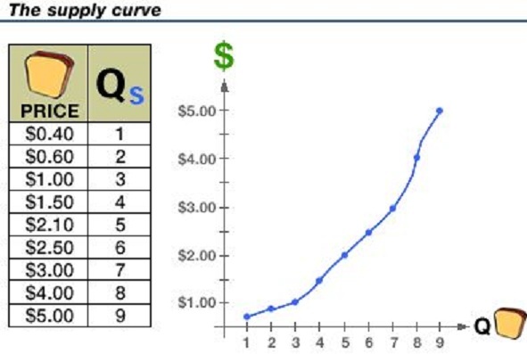
- The supply curve
- the supply schedule is a set of data
(table) showing the relationship between price and the
quantity supplied, ceteris paribus;
- low prices lead to low revenues, therefore less is
offered for sale by sellers
- high prices lead to high revenues and therefore
more is offered for sale by sellers
- convert the supply schedule into a supply graph
- always label the axes
- quantity on horizontal axis and price on the
vertical axis
- plot the data and connect the dots
- ME: the study guide has problems where YOU
can do the actual graphing; if graphs confuse or
worry you then you should do these
problems
- the supply curve shows the graphical
relationship between the price of a good and the
quantity supplied, ceteris paribus
|
|
- The law of supply
- supply curves slope upward this indicates a direct
relationship between price and quantity supplied
- the law of supply states that as the price of a good
or service increases, the quantity offered for sale generally
increases
- Rationale behind the law of supply
- ME: we will always explain the shape of the graphs that we
draw; we have already done this with the production
possibilities curve and with the demand curve; make sure you
understand the shapes of all the graphs in this
course.
- the law of increasing opportunity costs helps
explain the law of supply
- opportunity cost is the best alternative that is
given up; when a choice is made
- the more bread that a baker offers for sale, the higher
the cost of producing each additional loaf
- Why?
- the supply curves slopes upwards because the opportunity
costs rise as the business produces more and more, so they will
need a higher price or they will decide to do something
else
- also, we will see in a later video lecture that the supply
curve slopes upwards because the marginal costs (the extra
costs of producing one more, increase
- ME: the textbook offers these explanations for the law of
supply:
- higher prices mean higher revenue for the producer which
is an incentive for he producer to produce more
- as quantity increases the added cost of producing one
more unit of output (called the marginal cost) increases
because the factory will start to get crowded
- finally, I like to add the law of increasing cost that
we used to explain the shape of he production possibilities
curve, since all resources are not eh same as we increase
production of a good we will have to use less suitable
resources (like less qualified workers) which ill increase
coses. so, businesses will not produce more at a higher cost
unless they can get a higher price to cover those higher
costs
3.2-3 [TW 2.2.3
(6:52)] Understanding a change in Supply versus a Change in
Quantity Supplied - 3b
- Outline:
- Reviewing supply
- Supply and changes in the input prices
- Graphing a change in supply
- Change in quantity supplied vs. change in
supply
- Reviewing supply
- when we drew the supply curve we saw how the quantity
produced changed as we changed the price, ceteris
paribus
- ceteris paribus means that we held constant
everything else; only the price and quantity changed
- determinants that were held constant"
- Pi, T, G, Ex
- ME: Pe, Pog, Pres, Tech, Tax, Nprod
- but what happens if these other factors (ME: our textbook
calls these the "non-price determinants of supply")
change?
- in this lessen we will only look at a change in input
(resource) prices, then int he next video lecture will will
look at the other factors (determinants) of supply
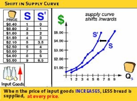
- Supply and changes in the input prices (price of
resources)
- what happens if the price of resources used to
produce the good (inputs) increase?
- profit will go down
- and businesses will produce less
- on the supply schedule we will see a smaller
quantity supplied AT EVERY PRICE;
- so on the supply schedule we will see lower
quantities supplied; at each price the quantity
supplied is lower; there is a new supply
schedule
- Graphing a change in supply
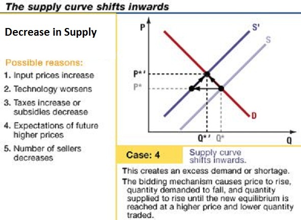
- so if the price of inputs goes up, this will cause
the supply curve to shift (move) to the left
- so on the supply curve there is a new supply
curve further to the the left; the supply has
DECREASES (shifted to the left)
|
|
- Change in quantity supplied vs. change in supply
- A change in the price of bread will cause a change in
quantity supplied which is a movement along a single supply
curve
- if one of the non-price determinants of supply change then
we get a whole new supply curve and we call this a change in
supply
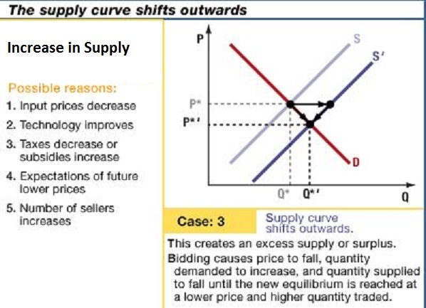
- an increase in supply means the supply curve
shifts to the left
- a decrease in supply means the supply curve
shifts to the right
3.2-4 [TW 2.2.4
8:47)] Analyzing Changes in Other Supply Variables - 3b
- Outline:
- Factors that influence producer's behavior
- Changes in the price of the product
- Changes in variables held constant when drawing the
supply curve
- VIDEO: Pi, T, G, Ex
- ME: Pe (Ex), Pog, Pres (Pi), Tech (T), Taxes (G),
Nprod
- Factors that influence producer's behavior
- VIDEO: Qs = S(P, Pi, T, G, Ex )
- ME: Qs = S(P, Pe, Pog, Pres, Tech, Tax, Nprod)
- Changes in the price of the product
- if the price of changes then there is a movement ALONG the
supply curve because price is already on the vertical axis
- we call this a change in the quantity supplied
- Changes in variables held constant when drawing the supply
curve
- VIDEO: Pi, T, G, Ex
- ME: Pe (Ex), Pog, Pres (Pi), Tech (T), Taxes (G),
Nprod
- if there is a change in one of these variables them the
supply schedule changes and we get a whole new supply
curve
- we call this a change in supply
- Pi
(change in the price of resources or inputs; Pres)
- if the price of resources increases then costs
increase and supply decreases -- shifts to the
left
- if the price of resources decreases then costs
decrease and supply increases -- shifts to the
right
- NOTE: a shifting of the demand curve means the the
quantity changes AT EACH POSSIBLE PRICE
- an increase in supply means the quantity
supplied increases at each possible price and the supply
curves shifts to the right
- a decrease in supply means that the quantity
supplied at each possible price decreases and the supply
curve shifts to the left
("
"means "change in")
- T
(change in technology)
- if the technology improves then productivity
increases and costs of producing the product will decrease
and supply increases -- shifts to the right
- if the technology gets worse then productivity
decreases and costs of producing the product will increase
and supply decreases -- shifts to the left
- G
(changes in taxes and subsidies)
- if taxes increase then costs of production
increase and supply decreases -- shifts to the
left
- if taxes decreases then costs of production
decrease and supply increases -- shifts to the
right
- if subsidies increase then costs of production
decrease and supply increases -- shifts to the
right
- if subsidies decrease then costs of production
increase and supply decreases -- shifts to the
left
- Ex
(change in expected price; Pe)
- if sellers expect the price to increase in the
future then supply today will decrease -- shift to
the left
- if sellers expect the price to decrease in the
future then supply today will increase -- shift to
the right
- ME: Pog
(change in the price of other goods also produced by the firm)
- if a producer produces to different products, let's say
corn and soybeans, then if the price of corn
increases then producers will produce more corn and
the supply of soybeans will decrease -- shift to the
left; why plant soybeans if they can get a higher price for
their corn?
- if a producer produces to different products, let's say
corn and soybeans, then if the price of corn
decreases then producers will produce less corn and
the supply of soybeans will increase -- shift to the
right; they will be willing to sell more soybeans at each
possible price since profits from corn are lower
- ME: Nprod
(change in the number of producers)
- if the number of producers increases then supply
increases -- shifts to the right
- if the number of producers decreases then supply
decreases -- shifts to the left
3.2-5 [TW 2.2.5
(7:16)] Deriving a Market Supply Curve from Individual Supply
Curves - 3b
- Outline:
- Recall the supply function
- The market supply curve
- Recall the supply function
- VIDEO: Qs = S(P, Pi, T, G, Ex )
- ME: Qs = S(P, Pe, Pog, Pres, Tech, Tax, Nprod)
- The market supply curve
- market supply is the horizontal summation of all of
the individual supply curves in the market
- for the market supply schedule we add up the
quantities at each price for ALL PRODUCERS; prices stay the
same and the quantities are added together
- therefore the market supply curve will be further to
the right as we add more producers
- since the quantity is on the horizontal axis we call this
horizontal summation; prices stay the same and the
quantities are added together
- What will shift the market supply curve?
- answer: anything that shifts the individual supply
curves
- VIDEO: Pi, T, G, Ex
- ME: Qs = Pe, Pog, Pres, Tech, Tax, Nprod
- ME:
- REMEMBER: a change in the price of the product itself
will NOT shift (change) the supply curve
- if the price of corn increases what will happen to the
supply of corn? Answer: NOTHING
3c - MARKET
EQUILIBRIUM and EFFICIENCY
- 3c PUTTING SUPPLY AND DEMAND TOGETHER - MARKET EQUILIBRIUM
- 3.3-1 Determining a Competitive Equilibrium [TW 2.3.1
(11:04)]
- 3.4-1 Defining Comparative Statics [TW 2.3.2
(7:02)]
- 3.4-1 Classifying Comparative Statics (should be 3.4-2, but
the link works) [TW 2.3.3 (13:04)]
- 3c MARKETS AND EFFICIENCY
3.3-1 [TW 2.3.1
(11:04)] Determining a Competitive Equilibrium - 3c
- Outline:
- Definition of competitive equilibrium
- Excess demand
- The bidding mechanism
- Excess supply
- A competitive equilibrium
- Definition of competitive equilibrium
- we will be putting what we have learned about demand and
supply together to create a model that will help us to predict
how factors in the environment will affect the price of a
product
- why are prices what they are and what makes price
change?
- competitive equilibrium:
- assumptions:
- there are many buyers and sellers in the market
- who have no influence over the price; i.e. they are
price takers
- competitive equilibrium occurs at the price where
the quantity supplied equals the quantity demanded
- equilibrium means that we have a situation in
which there is no tendency to change; a situation in which
neither consumers or firms have any incentive to change
their behavior
- there will be only one price in which there is no
pressure for something to change and that is the price where
the quantity demanded (Qd) equals the quantity supplied
(Qs); Qd=Qs
- graphically: the equilibrium will be the price where the
demand and supply curve cross; this is the price where
Qd=Qs
- Excess demand
- if the price is below the equilibrium then the Qd
> Qs and there will be excess demand
- Excess demand is the difference between the Qd and
the Qs when consumers demand a greater quantity than the
suppliers are willing and able to supply; i.e. when the price
is below the equilibrium price
- if there is excess demand then there will be a
shortage
- The bidding mechanism
- if the price is below the equilibrium then the
excess demand this will cause the price to go up so this is not
the equilibrium
- this is called the "bidding mechanism"; this is the
process by which unsatisfied buyers try to change the price of
a good in order to guarantee that they are able to obtain it;
unsatisfied buyers will be willing to pay a higher price to get
the product
- Tomlinson uses the term "reservation price"
- the bidding mechanism will continue to drive the price up
until the Qs=Qd and there is no more excess demand
- Excess supply
- if the price is above the equilibrium price then the Qd
< Qs and there will be excess supply, or a
surplus
- excess supply (or a surplus) is the difference between the
quantity supplied and quantity demanded when producers supply a
greater quantity than consumers are willing to buy; i.e. if the
price is too high
- if there is an excess supply the bidding mechanism will
cause the price to fall as sellers try to sell off their
surplus
- as the price goes down the quantity demanded will increase
and the quantity supplied will decrease; this means we will
move down along the demand and supply curves until we reach the
price where Qd = Qs or where the curves cross
- A competitive equilibrium
- occurs at the price where the quantity demanded by buyers
and the quantity supplied by producers are equal
- now there is no excess demand and no excess supply; there
is no further tendency to change; equilibrium has been
reached
- on the graph the equilibrium will occur where the supply
curve and the demand curve intersect (cross)
3.4-1 [TW 2.3.2
(7:02)] Defining Comparative Statics - 3c
- Outline:
- Competitive Equilibrium
- Three steps to finding a new equilibrium when a
non-price determinant changes
- identify which side of the market is affected? (will
it change demand or supply?)
- how does the change affect the curve? (will demand or
supply increase [shift right] or decrease [shift
left]?)
- how does the equilibrium change? (use the graph to
see what happened to the equilibrium price and
quantity)
- ME: Our textbook does not use the term "comparative statics",
but instead uses the term "equilibrium" which is also used in the
video lectures
- Competitive Equilibrium
- equilibrium occurs at the price where the Qs = Qd
- equilibrium will be at the price and quantity where the
supply and demand curves cross
- Three steps to finding a new equilibrium when a non-price
determinant changes
- we can use our model (graph) to predict, or explain, how
something in the environment (real world) affects the
equilibrium price and quantity of a product
- anytime that there is a change in one of the non-price
determinants of demand or supply then there will be a change
int he equilibrium price and quantity
- Tomlinson says that there are three steps:
- identify which side of the market is affected? (will it
change demand or supply?)
- how does the change affect the curve? (will demand or
supply increase [shift right] or decrease [shift
left]?)
- how does the equilibrium change? (use the graph to see
what happened to the equilibrium price and quantity)
- ME: Four steps
- first determine which non-price determinant has changed
- there are five non-price determinants of demand: Pe,
Pog, I, Npot, T (P, P, I, N, T)
- there are six non-price determinants of supply: Pe,
Pog, Pres, Tech, Tax, Nprod (P, P, P, T, T, N)
- if one of these 11 determinants change then we will
get a change in the price and quantity of the
product
- identify which side of the market is affected? (will it
change demand or supply?;
- did a non-price determinant of demand change? or
- did a non price determinant of supply change?
- will demand or supply increase [shift right] or
decrease [shift left]?
- how does the equilibrium change?
- GRAPH IT!
- then use the graph to see what happened to the
equilibrium price and quantity)
- do not try to guess; draw the graphs and shift
a curve and then you can see what happens to the
equilibrium price and quantity
- example:
- what would happen to the price of bread and the quantity
sold if the price of bagels, a substitute good, increases;
price of bagels goes up so what happens to the market for
bread?
- 4 steps:
- first determine which non-price determinant has changed
- demand: Pe, Pog, I, Npot, T
- supply: Pe, Pog, Pres, Tech, Tax, Nprod
- the non-price determinant that has changed is: POG -
substitute
- will it change demand or supply?
- since price of substitutes is a determinant of
demand, then the demand curve will shift
- how does the change affect the curve?
- we have learned that if the Pog-sub goes up
this will increase demand for our product
- price of bagels increasing will cause the demand
for bread to increase
- how does the equilibrium change?
- GRAPH IT!
- shift the demand to the right
- at the original price and with the new demand curve
we can see that there will now be excess demand
(Qd>Qs); this will create and excess demand and the
bidding mechanism will bid the price up
- from the graph we can see that if the price of
bagels increases this will cause the price
of bread to increase AND people will buy more
bread
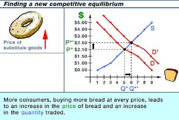
3.4-1 [TW 2.3.3 (13:04)] Classifying Comparative
Statics (should be 3.4-2, but the link works) - 3c
- Outline:
- Comparative statics
- The demand curve shifts outward (increase in
demand)
- The demand curve shifts inwards (decrease in
demand)
- The supply curve shifts outwards (increase in
supply)
- The supply curve shifts inwards (decrease in
supply)
- ME: Our textbook does not use the term "comparative statics",
but it does discuss how the non-price determinants of demand and
supply affect the equilibrium price and quantity and that is what
the video lecture does here
- Comparative statics
- comparative statics is comparing one state (condition) of a
competitive equilibrium to another when one of the variables
affecting demand or supply changes
- ME: NOTE --
- Goal: to see what happens to the price of a good and the
quantity traded (sold) when we change one of the variables
that we usually hold constant when drawing the supply and
demand curves
- there are only four possibilities:
- The demand curve shifts outward (increase in
demand)
- The demand curve shifts inwards (decrease in
demand)
- The supply curve shifts outwards (increase in
supply)
- The supply curve shifts inwards (decrease in
supply)
- ME: but more than one variable could change at the same
time including one or more of demand and one or more of supply;
our textbook has example of these
- The demand curve shifts outward (increase in demand)
- demand shifts to the right causing the price to increase
and the quantity to increase
- results in a shortage of the good at the original
price
- the price and quantity sold will increase
- what could cause an increase in demand?
- The correct change in the textbook's non-price
determinants of demand:
- Pe = expected price
- Pog = price of other goods including the price of
complements and the price of substitutes
- I = income
- Npot = the number of potential consumers
- T = tastes and preferences
- KNOW THESE!!
- The demand curve shifts inwards (decrease in demand)
- demand shifts to the left causing the price to decrease
and the quantity to decrease
- What would cause a decrease in demand?
- The supply curve shifts outwards (increase in supply)
- supply shifts to the right causing the price to decrease
and the quantity to increase
- This would cause a surplus and the price will begin to
drop
- What would cause an increase in supply?
- The correct change in the textbooks non-price determinants
of supply
- a change in the expected price (Pe,)
- a change in the price of another good also produced by
the firm (Pog)
- a change in the price of resources (Pres)
- a change in technology (Tech,)
- a change in taxes or subsidies
- a change in the number of producers (Nprod)
- KNOW THESE!
- The supply curve shifts inwards (decrease in supply)
- supply shifts to the left causing the price to increase
and the quantity to decrease
- What would cause a decrease in supply?
- KNOW THESE!
3c - MARKETS AND EFFICIENCY
Consumer and Producer
Surplus in the Linear Demand and Supply Model (10:01) - 3c
Free at: http://www.econclassroom.com/?p=2599
- Me:
- in chapter 1 we learned of the 5 ways to reduce scarcity
(the 5Es)
- in chapter 1 we also learned that benefit cost analysis
(marginal analysis) can be used to make good decisions
- in chapter 2 we learned that market economies tend to do
well at reducing scarcity because they tend to achieve
allocative and productive efficiency
- In chapter 3 we learned that in competitive market
economies prices are determined by demand and supply
- Here we will put it all together to see why market
economies achieve allocative efficiency
- we will use two models to show why competitive market
economies achieve allocative efficiency
- benefit cost analysis (marginal analysis)
- consumer and producer surplus
- consumer surplus is the extra benefit enjoyed by
the consumers in a market who pay less for a product than they
were willing and able to pay for it
- the demand curve also represents the marginal benefit of
all the consumers in this market: D=MB
- ME: our textbook uses the term Marginal Social Benefit
(MSB) to measure the MB
- remember the demand curve is downward sloping because of
diminishing marginal utility (MU = MB)
- ME: the price the consumers are willing to pay for a
product represents the benefits that they expect to get from
it. If you get a lot of benefit from something (like skiing in
Colorado) you would be willing to pay a higher price than you
would for something that gives you less benefits (like skiing
in Wisconsin)
- the area below the demand curve, but above the equilibrium
price, represents the total extra benefit of all the
consumers in a market, called consumer surplus
- calculate the area of the consumer surplus triangle to get
the numerical measure of consumer surplus
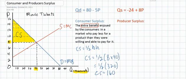
- producer surplus is the extra benefit enjoyed by the
producers in a market who sell their product for more than they
are willing and able to sell if for
- the supply curve also represents the marginal costs of all
of the producers in the market: S = MC
- ME: our textbook uses the term Marginal Social Cost (MSC)
to measure all of the MC of production
- remember the points on the supply curve shows the various
prices that firms are willing and able to offer their product
for sale
- you can see that there are points on the supply curve that
are below the equilibrium price.
- the difference between what a firm is willing to sell and
product for (the supply curve) and what they can sell it for
(the equilibrium price) is the consumer surplus
- the area above the supply curve, but below the equilibrium
price, represents the total extra benefit of all the sellers
in a market, called producer surplus
- calculate the area of the producer surplus triangle to get
the numerical measure of consumer surplus
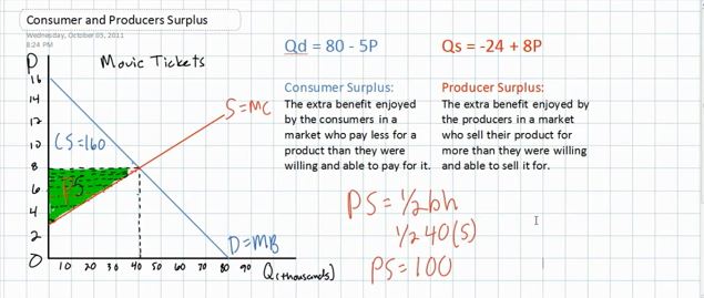
- allocative efficiency
- we can see that at the equilibrium price in a competitive
market the total surplus (benefits) is maximized; that is, the
total of consumer surplus and producer surplus is as large as
possible
- what if the price is NOT at the equilibrium?
- if the price is greater than the equilibrium then
producers would want to sell more BUT consumers will buy
less, and the total surplus to society will be less
- we can show the loss of satisfaction to society on the
graph (purple triangle)
- ME:
- this is called the dead weight loss
- this is not allocatively efficient; society is not
maximizing its satisfaction
- also you can see that at the higher price and lower
quantity the MB > MC (or MSB > MSC); we learned in
chapter 1 that if the MB > MC then we want more; we
gain more than it costs us so our satisfaction will
increase
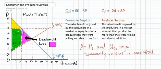
Supply, Demand, and Economic
Efficiency - 3c
Read: http://www.harpercollege.edu/mhealy/eco211/lectures/s%26d/sdeff.htm
Efficiency and Equilibrium
in Competitive Markets (11:48) - 3c
Free at: http://www.econclassroom.com/?p=2611
assumes knowledge of consumer and producer surplus, also uses benefit
cost analysis
- Efficiency exists in a society when no individual in
society can be made better off without making someone else worse
off
- Allocative efficiency occurs when the MB = MC (MSB = MSC)
- the demand curve is downward sloping indicating that society
is getting less extra satisfaction (MB) from consuming more
- the supply curve is upward sloping since the MC of producing
more goes up as resources become more scarce (ME: AND as we need
to use less suited resources to produce our product)
- Allocative efficiency occurs at the equilibrium price and
quantity because the total of consumer and producer surplus is
maximized at the equilibrium; ME: this is also where the MB = MC
(MSB = MSC)
- what if the quantity is less than the equilibrium quantity?
- we get allocative inefficiency because the MSB >
MSC
- we say that we have an underallocation of resources;
too few resources are being used to produce the product; we are
getting a lot of benefits (MB is high) and the costs to
society is low (MC is low)
- this means we want more or we would be happier if we had
more
- there is also a loss of total surplus to society; even
though producer surplus may increase, consumer surplus
decreases a lot and there is a loss to society, called the
dead weight loss (or welfare loss; "welfare" means
satisfaction)
- society is less satisfied and we have allocative
inefficiency
- what if the quantity was greater than the equilibrium
quantity?
- we get allocative inefficiency because the MSB <
MSC
- we say that we have an overallocation of resources;
too many resources are being used to produce the product; we
are getting few benefits (MB is low) and the costs to
society is high (MC is high)
- this means we want more or we would be happier if we had
less of this product (and more of something else that makes us
happier)
- there is also a loss of total surplus to society; the
dead weight loss (or welfare loss)
- in order to get producers to produce more they would need a
higher price
- this would decrease consumer surplus and even though
producer surplus would go up a little th3ere is a net loss to
society, the dead weight loss
- in a market economy society's satisfaction is maximized at the
equilibrium price and quantity
- ME:
- of course the equilibrium price ans quantity is WHAT WE
GET, because it is here that producers will make the biggest
profit
- the allocatively efficiency quantity is WHAT SOCIETY WANTS
because they maximize their satisfaction
- in a competitive market economy (with no externalities --
chapter 5) WHAT WE GET = WHAT WE WANT and we achieve allocative
efficiency
- This is the "invisible hand" of capitalism that
Friedman discussed in the previous video in chapter 2
[Power
of the Market (YouTube LibertyPen 1:14)]
- ME: our textbook shows the dead weight loss that results from
overproduction a little differently than does the video (see page
98 and the figure below)
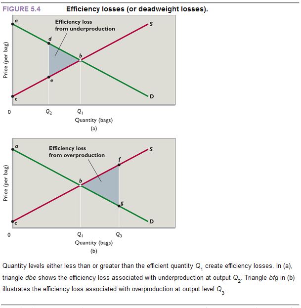
Chapter 5 - Market Failures and Externalities
(Modules 5a and 5b)
MODULE 5a - GOVERNMENT INTERFERENCE IN MARKETS and
NEGATIVE EXTERNALITIES
- GOVERNMENT INTERFERENCE IN MARKETS: Price Ceilings and Floors
- MARKET FAILURE:NEGATIVE EXTERNALITIES
- 14.1-1 Defining Externalities (negative externalities)
[TW 8.4.1 (5:46)]
- 14.3-1 Explaining How to Internalize External Costs
(Negative Externalities) [TW 8.4.2 (11:58)]
- 14.4-1 Finding a Market Solution to External Costs [TW
8.5.1 (12:21)]
- Introduction
to Market Failure and Negative Externalities of Production
(econclassroom.com 14:45)
- 14.4-2 Finding a Negotiated Settlement to an External Cost
-- the Coase Theorem [TW 8.5.2 (12:45)]
- 14.4-3 Applying the Coase Theorem [TW 8.5.3
(7:02)]
GOVERNMENT INTERFERENCE IN MARKETS: Price Ceilings and Floors
4.1-1 [TW 2.5.1 (9:38)] Understanding How Price
Controls Damage Markets (Price Ceilings) - 5a
- Outline:
- Price controls in rental housing
- Reduction in supply (error -- they really mean a
reduction in the QUANTITY SUPPLIED)
- Non-price competition
- Deadweight loss and rent-seeking
- Price controls for concert tickets
- Price controls in rental housing
- why put on a price control below the equilibrium price? --
to help the poor
- graph
- effects
- cheating and they avoid the rent controls
- a shortage caused by the reduction in the
quantity supplied and and increase in the quantity
demanded
- dead weight loss for society; allocative
inefficiency
- rent seeking = non-price competition
- Reduction in QUANTITY SUPPLIED (slight error on the video)
- fewer apartments will be available at the low
government-set price
- Deadweight loss and rent-seeking
- the Qd > Qs and we have a shortage (excess demand)
- usually the bidding mechanism will cause the price to go
up
- but the price cannot legally be raisedc above the ceiling
price
- The video lecture will ask you a
multiple choice question. ANSWER THE QUESTION by selecting A,
B, or C and more of the lecture will follow
- non-price competition
- people who want an apartment will need to do all kinds
of other things to compete for the few apartments available
which will cost the apartment seekers more
- using more resources but not giving society any
additional value
- both consumer and producer surplus are decreased and
society losses the deadweight loss AND the rent seeking
activities
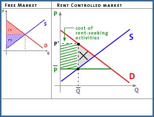
- Price controls for concert tickets
- shortage of tickets
- loss to society:
- standing in line
- scalpers
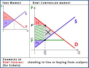
- putting on price controls does not help the poor
- the rich can afford to buy from scalpers
- price controls rarely achieve their goal
4.1-2 [TW 2.5.2
(14:47)] Understanding the Problem of Minimum Wages in Labor
Markets (Price Floor) - 5a
- Outline:
- Unintended consequences
- The supply and demand curves
- Substitution effect and income effect
- Minimum wage with supply and demand
- Unintended consequences
- Goal: to raise the income of unskilled workers
- but does it actually harm low wage workers?
- The supply and demand curves
- price = hourly wage
- quantity is the quantity of labor supplied by workers or
demanded by employers
- Substitution effect and income effect
- when the wage rate declines more labor is hired (demand is
downward sloping)
- as labor gets less expensive the costs of production go
down and businesses will produce more which requires more
labor
- as labor gets less expensive employers will substitute
more labor in place of some other input, and employ more
labor
- when the wage rate increases more labor is supplied (supply
is upward sloping)
- controversial:
- substitution effect: work or pleasure? -- as
the wage rate increases the opportunity cost of leisure
increases and workers will substitute work for labor
- income effect: work or leisure? -- the effect
on worker behavior when incomes rise
- is wages increase workers may work less since now
workers can afford to pay bills by working fewer hours
and then take more leisure
- what would you do if your wage was doubled? -- work more
or work less?
- we'll assume that the substitution effect is stronger
and the supply of labor curve is upward sloping
- Minimum wage with supply and demand
- in a free market the equilibrium wage rate will occur where
Qs = Qd; where the curves cross
- what happens if the government sets a minimum wage rate
that is higher then the equilibrium?
- this is a price floor; the wage cannot go below
the minimum
- effects:
- the quantity supplied of labor will increase
because wages are higher and more people will want to
work
- the quantity demanded of labor is reduced
because a higher rage increases the costs of production
and businesses will produce less and need fewer workers
and the higher wage will encourage businesses to
substitute other resources in place of labor and
therefore fewer workers will be hired
- Unintended consequence:
- Qs > Qd and there is an excess supply of labor;
this is unemployment; the higher minimum wage
causes unemployment
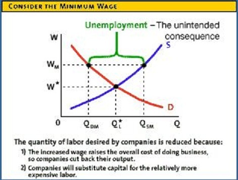
- since some workers are willing to work for less
than the minimum wage employers will be able to
pass some of the costs onto the workers
- dead weight loss for society; there are
jobs where the MB to society is greater then the MC
but because of the minimum wage they will not be
filled
- Note: if the minimum wage is set below the
equilibrium then it will have no effect because the
market forces will bid the wage up to the equilibrium; wages
can be higher than the minimum wage but not lower
- ME: the video shows that an effective minimum wage will
cause unemployment of unskilled workers, but it doesn't ask
HOW MUCH unemployment and HOW MUCH more will low-wage
workers earn? Do minimum wage laws help the poor or hurt the
poor?
- unemployment hurts the poor,
- but if only a little unemployment is created and the
vast majority of workers earn higher incomes then
overall, the wage income of the poor will increase. We
will discuss this in the chapter on
elasticity.
Determining the Effects of
Price Ceilings and Price Floors - 5a
http://www.econclassroom.com/?cat=13
- Price Floor is a minimum price for a good established
by the government at a level above the free market equilibrium
price (butter in Europe)
- the goal of a price floor is to raise the price to help the
producers
- therefore the Qs will increase (move along the supply
curve)
- and, the Qd will decrease (move along the demand
curve)
- result: a surplus will be created
- efficiency effects:
- consumers will buy less at the higher price and the
amount of consumer surplus will decrease
- since the quantity sold decreases, the producer
surplus does not increase by as much as we might
expect
- net effect of the price floor:
- dead weight loss of satisfaction (or welfare)
to society
- allocative inefficiency: ether will be an
overallocation of resources but the quantity
demanded by consumers will be lower
- this creates a surplus
- ME: Note: if the price floor is set below the
equilibrium then it will have no effect because the market
forces will bid the price up to the equilibrium; prices can be
higher than the price floor but not lower
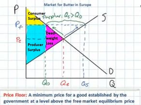
- Price Ceiling is a maximum price for a good established
by the government at a level below the free market equilibrium
price (gasoline [petrol] in China)
- the goal of a price ceiling is to reduce the price to help
the consumer
- therefore the Qd will increase (move along the demand
curve)
- and, the quantity supplied will decrease (move along the
supply curve)
- resulting is a shortage since the Qd > Qs
- efficiency effects:
- the actual quantity available will be less
- this will increase consumer surplus, but not by
as much as we might expect due to the lower quantity
available
- producer surplus is less due to the lower price
- there is a dead weight loss of satisfaction for society
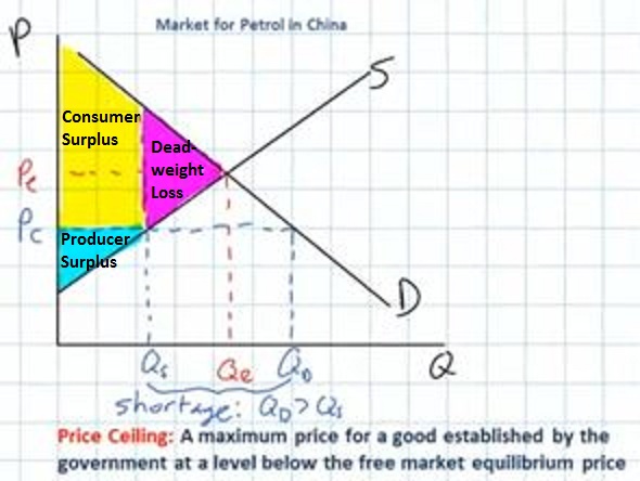
- ME: Note: if the price ceiling is set above the
equilibrium then it will have no effect because the market
forces will only bid the wage up to the equilibrium; prices can
be lower than the price ceiling but not higher
- Summary:
- a price floor reallocates welfare (satisfaction) from
producers to consumers but overall causes a net loss of
satisfaction, i.e. allocative inefficiency, since there is a
surplus; an overallocation of resources
- a price ceiling reallocates welfare (satisfaction) from
consumers to producers but overall causes a net loss of
satisfaction, i.e. allocative inefficiency, since there is a
shortage; an underallocation of resources
MARKET FAILURE:
EXTERNALITIES
Negative
Externalities
14.1-1 [TW 8.4.1
(5:46)] Defining Externalities - Negative Externalities -
5a
- Outline:
- Definition of Externalities
- External Costs (also called Negative Externalities or
Spillover costs)
- External Benefits (also called Positive Externalities or
Spillover Benefits)
- The Problem with Externalities
- if there are positive externalities - Definition of
Externalities
- ME: in a previous lesson we learned that a competitive
market economy achieves allocative efficiency. Adam Smith
called this the "invisible hand" of capitalism. We said "what
we get = what we want". A market failure occurs when the
market does not achieve allocative efficiency
- an externality is a cost or a benefit that can be
passed on to others
- External Costs (also called Negative Externalities or
Spillover costs)
- an external cost (or negative externality or spillover
cost) is a cost of a transaction that is borne by someone who
is not a party to that transaction; not the buyer and not the
seller, but someone else must pay part of the cost of the
transaction
- examples: pollution created by the production of a product;
second hand smoke from cigarettes; painting your house an ugly
color makes your neighbors "
- External Benefits (also called Positive Externalities
or Spillover Benefits)
- an external benefit (or positive externality or spillover
benefit) is a benefit of a transaction that is received by
someone who is not a party to that transaction; not the the
buyer and not the seller, but someone else benefits without
paying
- examples: you get a flu shot and others around you are
protected from getting the flu from you, they benefit from you
getting the shot
- The Problem with Externalities
- Market failure occurs -- the free market does
not produce the quantity that maximizes society's satisfaction
= allocative inefficiency
- we saw in previous lectures that usually supply and demand
in a market economy has the result of producing the
allocatively efficient quantity; what we get = what we
want
- a private business will look at the marginal benefits and
the marginal costs of producing more and will produce as long
as the MB > MC, BUT when there are negative
externalities the costs to the firm are less than the total
costs to society since they can avoid some costs by passing
them on to others. the result is too much will be
produced = an overallocation of resources
- if there are positive externalities consumers look
at the MB and MC. BUT they do not include all of the benefits
since some of the benefits have spilled over onto some one
else. The result is the consumers see lower benefits that
society does and too few will be consumed = an
underallocation of resources
Internalizing an
Externality
14.3-1 [TW 8.4.2
(11:58)] Explaining How to Internalize External Costs (Negative
Externalities) - 5a
- Outline:
- How negative externalities cause market failure
- How to correct for that market failure
- How negative externalities cause market failure
- assume you have a company that causes a pollution when it
produces its product (boxes)
- then the private costs to the firm are less than the
true social costs of production
- how do we calculate these external cost?
- measure the costs of how much it would cost to
prevent the pollution
- or how much it would cost to clean up the
pollution
- or how much you would have to pay the people who
suffer from the pollution to accept it
- economists will measure these external costs by choosing
the least expensive measure
- result:
- from the viewpoint of society all quantities should
be produced as long as the MB are greater than the
marginal social costs (the private costs plus the
external costs
- from viewpoint of the producer they will continue to
produce as long as the MB are greater then just the
private costs
- the result will be that the producer will produce
MORE THAN the optimal quantity for society. We call this
an overallocation of resources. the market failed to
achieve allocative efficiency.
- How to correct for that market failure
- the principle of the second best: the best method to be
used in a market failure is the one that most precisely
corrected for the original problem
- although it would be best if there were no negative
externalities then businesses would produce the allocatively
efficient quantity and society's satisfaction is
maximized,
- but if there are negative externalities then the second
best solution or society is to find a method that best
approximates the efficient outcome
- we call this "internalizing the externality": make
the producer pay the external costs; then the total private
costs will be the same as society's costs
- How?
- by putting a tax on the seller for each one that they
produce that is equal to the size of the external costs
- since this will raise the producer's costs, they will
produce less
14.4-1 [TW 8.5.1
(12:21)] Finding a Market Solution to External Costs - 5a
- Outline:
- Supply and demand diagrams
- Correcting the externalities
- Applying the principle of the second best
- Re-creating a missing market
- Quick review
- Supply and demand diagrams
- if the demand represents marginal social benefits (MSB) and
the supply equals marginal social costs (MSC) then the
equilibrium quantity that we get (where Qs = Qd) will be the
same as the allocatively efficient quantity that we want (where
MSB = MSC); i.e.when there are no externalities, markets
achieve allocative efficiency
- ME: when Tomlinson talks about maximizing economic
value I use the term achieve allocative
efficiency (which is producing the quantity that
maximizes society's satisfaction [value])
- but what happens if there are negative externalities, or
external costs, that the firm does not have to pay?
- if there are negative externalities than the private
costs to the firm are not the same as the costs to
society
- Tomlinson uses the term "reservation price" which is the
highest price a buyer is willing to pay for a good or
service. This reservation price is a measure of the marginal
benefits that the buyer receives
- the supply curve for the business will be to the left
(below) the costs to society (MSC) because since the firm
avoids paying hate external costs their costs are lower and
when costs go down we know that supply goes up (shifts to
the right)
- the vertical distance between the MSC curve and the
supply curve is the value of he external costs
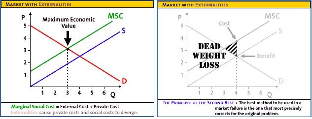
- quantity 3 is the allocatively efficient quantity; what
we want
- quantity 4 is the profit maximizing quantity; what we
get
- if there are negative externalities then too much will
be produced (overallocation of resources) resulting in a
loss of satisfaction to society = dead weight loss =
allocative inefficiency
- Correcting the externalities
- to make the producer internalize the externality we could
tax them. a tax on the product will decrease the supply and
cause the profit maximizing quantity to decrease.
- if the tax is equal to the value of the external cost then
the producer's supply curve will become equal to the MSC curve
and allocative efficiency will be achieved
- Applying the principle of the second best
- find out what the problem is then find a policy that will
precisely as possible offset the original problem
- like a tax on boxes if the production of boxes cause
pollution
- Re-creating a missing market: a tax on pollution
- but boxes are not the problem, pollution is the
problem
- so we could get a similar outcome if we could tax producers
for the pollution; this would also increase their costs and
they will produce less -- and pollute less
- but they could also try to find a way to pollute less so
that they will not have to pay as much pollution tax, This is
good for society AND it would not occur if we taxed the
boxes
- how do you calculate a pollution tax?
- you could do scientific studies to estimate the social
costs of the pollution
- OR you can set up a market for pollution permits
- the buying and selling of these pollution permits will
result in a market price for them
- to avoid paying for pollution permits firms will try to
reduce pollution
- or environmental groups may buy some of he permits and
not use them to reduce pollution even more
- problem with an externality is that there is a missing
market like a market for pollution
- Quick review
Introduction to Market
Failure and Negative Externalities of Production
(econclassroom.com 14:45) - 5a
http://www.econclassroom.com/?p=2850
- A Market Failure exists whenever the free market
equilibrium quantity of output is greater or less than the
socially optimal (also called "allocatively efficient")
level of output. the free market will produce either too much or
too little.
- failed to achieve the socially optimal, or allocatively
efficient, level of output.
- but what is the allocatively efficient level of output
- graph:
- supply represent the marginal costs of production
- demand represents the marginal benefits that consumers
receive (ME: if there are no positive externalities then d=MSB
[marginal social benefit]
- Negative externalities (also called spillover costs and
external costs)
- exist whenever the production of a good creases spillover
costs for society that are not born by the producer of the
good;
- MPC (marginal private cost) are the costs paid by
the producer of the product
- MSC (marginal social cost) are all the costs to
society including the MPC plus any external costs (negative
externalities)
- MPB (marginal private benefits) are the benefits
received by the buyers of the product
- MSB (marginal social benefits are all of the
benefits to society from the production and consumption of a
product including the MPB plus any external benefits (positive
externalities)
- graph: when there are negative externalities then the firm
AVOIDS some costs so the costs to the firm are lower; therefore
the MSC are greater than the MPC
- examples: if the production of a good creates pollution
that the firm does not need to clean up; health costs that the
firm can avoid paying
- the point is the MSC > MPC
- the socially optimum quantity (or the allocatively
efficient quantity) occurs where MSC = MSB; the is WHAT
WE WANT
- the equilibrium quantity (the profit maximizing
quantity) occurs where Qd = Qs; this is WHAT WE GET
- you can see on the graph that when there are negative
externalities the producers will produce too much, the profit
maximizing quantity that we get is greater than the
allocatively efficient quantity that we want; we say that there
is an overallocation of resources
- ether is a dead weight loss to society; less
satisfaction for society; if less was produced then society
would be better off (have more satisfaction)
- what can the government do to increase society's
satisfaction?
- usually when the government gets involved in the market
id causes inefficiency (less satisfaction)
- but when there are negative externalities the market
itself is inefficient (too much is being produced) and the
government might be able to make it more efficient
- an excise tax is a per unit tax on the
production of a good; we should know that a tax is a
non-price determinant of supply and when the tax goes up,
costs go up and supply goes down
- if the government can set the tax exactly equal to
the size of he per unit external costs then the supply
curve will move back to the MSC curve.
- then, with the tax, the profit maximizing quantity
that we get (where Qd = Qs) will be the same as the
allocatively efficient quantity (where MSB = MSC) that we
want
- consumer surplus, producer surplus, and tax
revenue
- a tax on the production of goods that creates
negative externalities is a corrective tax that increases
society's welfare (satisfaction gained = purple
triangle;) allocative efficiency is increased
Coase Theorem
14.4-2 [TW 8.5.2
(12:45)] Finding a Negotiated Settlement to an External Cost -
5a
- Outline:
- Government action vs. bargaining
- 2 companies operating independently
- 2 companies cooperating
- Definition of the Coase Theorem
- Government action vs. bargaining
- Review: when there are negative externalities the
government can correct for the overallocation of resources by
taxing the production or regulating the producers
- here we explore the Coase Theorem that says that under
certain circumstances bargaining can solve the problems created
by negative externalities without the government
- Example:
- boxes have a price of 50 cents which represents the
marginal social benefit (MSB)
- box producer pollutes lake and saves 25 cents per
box
- beers have a price of $1 which represents the marginal
social benefit (MSB)
- beer brewer uses water from the lake for free, but if
the lake is polluted by the box maker then it costs the
brewer 50 cents to clean the water before making the
beer
- 2 companies operating independently -- if the box maker and
beer brewer are acting independently
- then the box maker will pollute the lake to make greater
profits (profits = 50 cents)
- the beer brewer will then have to spend 50 cents per beer
to clean the water and profits will be 50 cents
- total profit = 50 cents + 50 cents = $1.00
- 2 companies cooperating
- What if they cooperate (work together)? could they find a
solution that benefits them both?
- Since it costs the box maker only 25 cents not to pollute,
but it costs the beer brewer 50 cents to clean the polluted
water before brewing the beer
- What if the beer brewer offers to pay the box maker the 25
cents that it would cost not to pollute in the first place?
- then the beer brewer is earning a bigger profit of 75
cents ($1 price minus 25 cents to pay the boxmaker not to
pollute
- and the beer brewer could then use some of that extra
profit to encourage the box maker to go along with the
deal.
- the box maker says that as long as the brewer is paying me
the 25 cents that it costs to clean up my pollution PLUS a
little extra, then they gain from cooperating
- RESULT: they both come out ahead since the total profits
are higher -- total profit = 50 cents for the box maker plus
75 cents for the brewer = $125
- it doesn't matter who owns the lake. The total economic
value will remain the same and the lake will not be polluted
only the distribution of the total economic value is affected
by ownership of the lake
- Definition of the Coase Theorem
- when two parties can get together with negligible cost,
then the result of that bargain will be one that maximizes
economic value of the situation
- also, then property ownership will not affect the outcome
of that decision
- only the distribution of the economic value will be
affected by property ownership
14.4-3 [TW 8.5.3
(7:02)] Applying the Coase Theorem - 5a
- Outline:
- Example of the Coase Theorem
- Example of additional parties
- When is government action necessary?
- Review of the Coase Theorem
- Example of the Coase Theorem
- benefit of a box (price) = $.50
- benefit of a beer = $1.00
- cost of cleaning up the pollution for the brewer = $.25
(lower than previous lecture)
- cost of preventing pollution to the box maker = $.50
- note: the cost to prevent pollution > the cost to the
brewer to clean it up
- when the lake is polluted the total profit = $.50 + $.75 =
$1.25
- if they try to negotiate:
- brewer is only willing to offer up to $.25 to the box
maker to have then not pollute
- but the box maker saves $.50 by polluting
- so they will be unable to reach an agreement
- total profit if the box maker pollutes = $.50 + $.75 =
$1.25
- total profit if the box maker does not pollute: $0 + $1.00
= $1.00
- result: more total profit if the lake is polluted
- so the Coase theorem still produces the result that
maximizes total value (satisfaction) for society
- Example of additional parties
- but what if other people (like swimmers) are also affected
by the pollution from the box maker
- a polluted lake will take satisfaction (value) from the
swimmers
- could they negotiate with the box maker not too pollute??
- they could, but
- if there are so many swimmers it might make it too
difficult; the transaction costs would be too high
- so they probably would not negotiate
- result: when there are too many parties involved making
hate transaction costs of private negotiations too high, there
will be no negotiations and the market will fail to maximize
society's satisfaction; allocative efficiency will not be
achieved
- When is government action necessary?
- when there are too many parties involved making hate
transaction costs of private negotiations too high a market
failure results and we will need government to correct for the
market failure
- government can force the box maker to clean up the
pollution to increase society's satisfaction
- Review of the Coase Theorem
- when two parties can get together, with negligible cost,
then the result of private bargaining will be one that
maximizes economic value for society
- also, the property ownership will not affect the outcome of
the negotiations; only the distribution of the economic value
will be affected by property ownership
- however, if the transaction costs are high, like if there
are many affected parties, then it may be better for society to
have the government help manage the externality
MODULE 5b -
POSITIVE EXTERNALITIES and PUBLIC GOODS
- MARKET FAILURE: POSITIVE EXTERNALITIES
- MARKET FAILURE: PUBLIC GOODS
14.3-2 [TW 8.4.3
5:34)] Explaining How to Internalize External Benefits (Positive
Externalities) - 5b
- Outline:
- External benefit and a market failure
- Subsidy correcting a market failure
- The principle of the second best
- External benefits and a market failure
- Get a flu shot? -- yes, as long as the MB>MC
- but the benefits of the flu shot to the individual do
not include the external benefits that the shot has on
society; so the benefits to the individual are less that the
total benefits and since the benefits are less there will be
fewer flu shots than the quantity that is best for
society
- there will be quantities where the marginal benefits to
society are greater than the marginal costs, and society
would gain if the person got the shot BUT since the
individual only looks at their private benefits which could
be less that the marginal costs and if MB<MC we will
choose not to do that thing
- Result:
- there will be too few flu shots from society's
viewpoint
- what we get < what we want
- dead weight loss to society
- External benefit and a market failure
- so what can be done?
- goal is to increase the quantity (have more people get flu
shots)
- Subsidy correcting a market failure
- a subsidy to the consumer will allow them to internalize
the external benefit
- give them money for getting a shot which will increase
their private benefits and more people will get shots
- if the subsidy make the private benefits equal to the
social benefits then the quantity of shots received will equal
the allocatively efficient quantity
- The principle of the second best
Market Failure: Positive
Externalities of Consumption (econclassroom.com 10:61) -
5b
http://www.econclassroom.com/?p=2871
- A positive externality occurs when the consumption of a
good or service creates benefits for society beyond those enjoyed
by the individual consumer
- when there is a positive externalities the MSB (all the
benefits that society, including the consumer, gets from that
product) are greater than the marginal private benefits (just the
benefits that the consumer gets.
- graph -- market failure:
- MPC (marginal private cost) are the costs paid by
the producer of the product
- MSC (marginal social cost) are all the costs to
society including the MPC plus any external costs (negative
externalities)
- MPB (marginal private benefits) are the benefits
received by the buyers of the product
- MSB (marginal social benefits are all of the
benefits to society from the production and consumption of a
product including the MPB plus any external benefits (positive
externalities)
- condoms have positive externalities:
- lower expenditures on public health due to the reduced
chance of STDs and fewer unwanted pregnancies
- lower population growth rate
- lower HIV infection rate leading to a more productive
workforce and more economic growth
- first we will assume that there are no external costs
(negative externalities) therefore the MSC = MPC (marginal
private costs or Supply)
- but the D=MPB which just measures the benefits going to the
people who use condoms
- the MSB curve includes the marginal private benefits
(people who use condoms are part of society) plus the external
benefits that spillover onto the rest of society (reduced
spread of STDs); so the MSB are greater than the MPB and the
graph is further to the right
- market failure :
- the equilibrium quantity (or profit maximizing quantity)
where Qs = Qd will be less than the allocatively efficient
quantity that maximizes society's satisfaction (the quantity
where MSB = MSC)
- too few will be bought; there will be an underallocation
of resources to condom production
- private individuals only look at there own private
benefits and maximize their personal satisfaction by
buying the equilibrium quantity
- but society's benefits (MSB) are greater because they
include the private benefits of the individual buying the
condom PLUS the external benefits discussed above; so the
socially optimum quantity (ME: which I like to call the
allocatively efficient quantity) is greater
- graph -- what can be done to correct the market failure?
- goal:
- to get more condoms
- to achieve allocative efficiency
- to maximize society's satisfaction
- what could be done?
- positive advertising to increase demand (MPB or
private demand) then more people will buy condoms
- subsidize the sale of condoms will increase
the SUPPLY of condoms (subsidy is a non-price
determinant of supply) which will lower the price and
increase the quantity demanded
MARKET FAILURE: PUBLIC
GOODS
15.1-1 [TW 8.2.1
(13:32)] Defining Public Goods - 5b
- Outline:
- What are public goods?
- Problems with public goods
- How can we correct for this market failure?
- What are public goods?
- we have said that if the market doesn't fail then the
market mechanism will result in a value (satisfaction)
maximizing solution for society; the best amounts will be
produced; we will get allocative efficiency
- if there are market failures then the market does not
achieve allocative efficiency; does not maximize society's
satisfaction (value)
- market failures include:
- negative externalities
- positive externalities
- public goods
- definitions:
- public goods are goods that when once they are
provided, people cannot be excluded from getting them; with
public goods you can get them even if you do not pay for
them
- with private goods (also called exclusive
goods) you don't get them unless you pay for them
- exclusive goods are goods that each consumer
must pay for to receive benefits (i.e. to get it)
- a rival good is one that when it is consumed by
one person it reduces the benefits of consumption for
another person, e.i. another person cannot also consume
it
- Problems with public goods
- the free rider problem
- the tragedy of the commons
- Examples:
- private goods (exclusive goods meaning that there is no
economically feasible way to exclude non-payers from getting
the good.)
- exclusive and rival: hamburger
- exclusive and non-rival: music download
(assuming that you pay for your music)
- RESULT: the market will allocate resources efficiency
and society's satisfaction will be maximized
- public goods (non-exclusive)
- non-exclusive and rival: a freeway or a park
- I can use it even if I do not pay for it
- but when I use it there is less room on the
freeway or in the park for other people
- this is called the tragedy of the
commons: the tendency of people to overuse a
public good because they do not have to pay for its
use
- one solution to the tragedy of the commons is to
create a market for these goods; we know that it IS
possible to prevent non-payers from using a highway or
a park; we call such roads "tollways" and many states
charge for using state parks, this will; this can
prevent their overuse; then these goods have become
private goods
- non-exclusive and non-rival: public
television, streetlights, national defense, roads,
lighthouse
- I can watch it even if I do not donate during the
pledge drives and once a streetlight is on there is no
feasible way to prevent someone from enjoying its
benefits
- and when I watch it you can also watch it
- free rider problem arises: some consumers can
receive the benefits without paying and therefore
fewer will be produced
- RESULT: the market will not allocate resources efficiency;
i.e. the market fails
- because of the free rider problem we may not get any
public goods (who is going to produce a product that
consumers can take without paying?)
- and if we do get a public good it tends to be
overused
- How can we correct for this market failure?
- Review:
- market demand for private good (exclusive) is the
horizontal summation of the individual demand curves: we add
all the quantities at each price
- Deriving the demand for a public good (non-exclusive)
- in a market for a public good we vertically sum the
individual demand curves
- this means at each quantity were add up the prices that
people are willing to pay
- our goal is to get a measure of the value, or
satisfaction, that society gets from each quantity
- and since once we have a certain quantity then the
satisfaction to society can be measured by how much each
consumer would have been willing to pay for that quantity if
they had to
- example: how much value does a street light provide?
- the demand (total social benefit) for a public good
is the vertical summation of the individual demand
curve
- What is the value maximizing quantity (socially optimum)
of streetlights? What quantity would be best for society?
What is the allocatively efficient quantity?
- where the MSB = MSC; this is the socially optimal
quantity
- the MSB is the demand curve for a public good
(vertical summation)Who is going to pay for the public
goods?
- Who is going to pay for the public goods?
- ideally, each consumer should pay for the benefit that
they get
- but. it may be difficult to determine each person's
benefit
- so, we need a second best solution: the government can
tax society and build streetlights for them
The Tragedy of the Commons
as a Market Failure (econclassroom.com 14:29) - 5b
http://www.econclassroom.com/?p=2945
- Natural resources which have no private owner or any system to
manage who has access to these resources
- Garrett Hardin interview
- reference to Karl Marx
- if common pasture land then too many people will use
it
- Two solutions:
- either divide it up (private property)
- or manage it jointly (socialism)
- Common access resources are natural resources over
which there is no private ownership established and no system for
managing the allocation of these resources
- Tragedy of the commons
- individuals will have an incentive to consume as many
common access resources as possible so that the competition
does not use them first
- private individuals will exploit common resources
unsustainably out of self-interest, ultimately leading to the
depletion of the resource
- this concept can be applies to: common pastures, seas,
forests, atmosphere
- graphical analysis of the tragedy of the commons
- market for fresh seafood assuming no limits on fishing
- D = MSB
- S = MPC
- but MPC < MSC
- so MSC lies above MPC
- because the social costs include all future costs of
seafood production
- and future costs will be higher if there re less fish in
the sea
- currently fish are being depleted unsustainably and
future costs to society, including future prices to
consumers, will be higher
- these then are external costs ((negative
externality)
- outcome: overallocation of resources
- the equilibrium quantity where Qd = Qs (profit
maximizing quantity, what we get) is greater then the
socially optimum quantity where MSB = MSC) (the allocatively
efficient quantity, what we want)
- too many fish will be consumed today this is the tragedy
of the commons
- same analysis could be applied to forest resources and even
the atmosphere
- too many forests are being cut today because current
costs do not account for future costs
- atmosphere: no private ownership and private costs of
using the atmosphere (like releasing pollution) are lower
than the social costs (air pollution, global warming) so too
much pollution is released
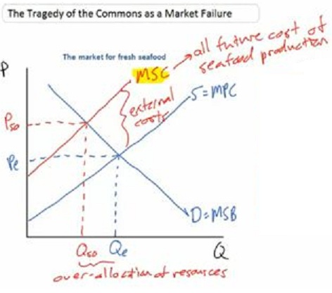
- So what can be done to internalize these externalities?
- Garrett Harding -- only two solutions exist:
- privatize
- manage as a group like the government (socialism)
- Privatize: Permits for usage
- fishing permits
- permits for pollution
- Public management
UNIT 2
Chapter 4 - Elasticity (Modules 4a and 4b)
MODULE 4a - PRICE ELASTICITY OF DEMAND AND TAX
INCIDENCE
- PRICE ELASTICITY OF DEMAND
PRICE ELASTICITY OF DEMAND
5.1-1 [TW 2.4.1
(4:47)] Defining Elasticity - 4a
- Outline
- Defining elasticity
- The effects of elasticity on total revenue
- Defining elasticity
- Will lowering the price of a good increase your
revenue?
- elasticity means "responsiveness"
- the elasticity of demand is the extent to which the
quantity demanded changes when there is a change in the price
of a good (ME: our textbook uses the term "price elasticity of
demand")
- the price elasticity of demand is the percentage
change in quantity demanded that results from a percentage
change in price
- ME:
- we know from chapter 3 that if price goes down then
quantity demanded (not demand) goes up, elasticity tells us
HOW MUCH the quantity demanded goes up
- if the P
 Qd
Qd or Qd
or Qd  ?
?
- if the price goes down, HOW MUCH does the quantity
demanded increase: a little or a lot?
- HOW MUCH will the Qd change when the price
changes?
- or
- if the P
Qd
 or Qd
or Qd  ?
?
- if the price goes up HOW MUCH does the quantity
demanded decrease: a little or a lot?
- HOW MUCH will the Qd change when the price
changes?
- The effects of elasticity on total revenue
- if at a price of $2, the quantity sold is 20
- if at a price of $1, the quantity sold is 30
- so when the price went down the total revenues (TR = P x Q)
went down. $2 x 20 = $40 and $1 x 30 = $30
- so when the price went down the quantity demanded went
up a little
- the demand curve is steeper
- demand is less elastic
- if at a price of $2, the quantity sold is 20
- if at a price of $1, the quantity sold is 50
- so when the price went down the total revenues (TR = P x Q)
went up. $2 x 20 = $40 and $1 x 50 = $50
- so when the price went down the quantity demanded went
up a lot
- the demand curve is flatter
- demand is more elastic
- what happens to total revenue when the price went
down?
- It depends on elasticity
- The video lecture will ask you a
multiple choice question. ANSWER THE QUESTION by selecting A,
B, or C and more of the lecture will follow
- inelastic demand (quantity demand is not very responsive to
a change in price)
- if at a price of $2, the quantity sold is 20, then total
revenue = P x Q = $2 x 20 = $40
- if at a price of $1, the quantity sold is 30 then TR= P
x Q = $1 x 30 = $30
- so when the price went down the quantity demanded went
up a little and the total revenue declined
- if demand is inelastic and the price goes down, then the
TR will decrease
- elastic demand (quantity demand is very responsive to a
change in price)
- if at a price of $2, the quantity sold is 20, then total
revenue - P x Q = $2 x 20 = $40
- if at a price of $1, the quantity sold is 50 then TR= P
x Q = $1 x 50 = $50
- so when the price went down the quantity demanded went
up a lot and the total revenue increased
- if demand is elastic and the price goes down, then the
TR will increase
5.1-2 [TW 2.4.2
(11:43)] Calculating Elasticity - 4a
- Outline
- Defining elasticity
- Characteristics of the formula for elasticity
- Calculating elasticity using the midpoint
formula
- Defining elasticity
- when we measure elasticity we want a formula that does not
depend on the units:
- this means it should not matter if we measure the price
of ice cream in dollars ($1) or in pennies (100 cents)
- and it should not matter if we measure the quantity of
ice cream in cones, or scoops, or pounds
- we want a unitless measure
- definition of the price elasticity of demand:
- Characteristics of the formula for elasticity
- Fraction
- the fraction bar means "that results from"
- Never negative due to the absolute value in the formula
- the two bars on each side of the formula mean "absolute
value"
- absolute value means that we ignore the negative
sign
- we know that there is an inverse relationship between P
and Qd
- this means that the fraction that we use when we
calculate the price elasticity of demand will always have a
negative value
- so the |absolute value bars| on each side
of the fraction just means that we get rid of the negative
sign
- Unitless measure
- by calculating PERCENTAGE CHANGES we get rid of the
units
- it doesn't matter whether we measure the price in
dollars or pennies, the percentage change will be the
same
- Calculating elasticity using the midpoint formula
- ME: YouTube
video on how to calculate percentages
- ME: our textbook calls this the "coefficient of price
elasticity of demand" (Ed)
- How to calculate a percentage change in quantity demanded
(%Qd)
- first you find the change in Qd by taking the new Qd
minus the old Qd
- then you divide by . . . .what?
- The video lecture will ask you a
multiple choice question. ANSWER THE QUESTION by selecting
A, B, or C and more of the lecture will follow
- usually the original (old quantity), BUT . . . WE WON'T
DO THIS. WE WILL USE THE MIDPOINT FORMULA, because if you
use the original quantity in the denominator you will get a
different percent change in quantity for price increases and
for price decreases
- Tomlinson says: "WAIT A MINUTE SOMETHING
IS WRONG HERE"
- we want one measure of elasticity that is the same for
price increases and for price decreases so we will use the
MIDPOINT on our graph for our denominator (what Tomlinson
calls the "base")
- The video lecture will ask you a
multiple choice question. ANSWER THE QUESTION by selecting
A, B, or C and more of the lecture will follow
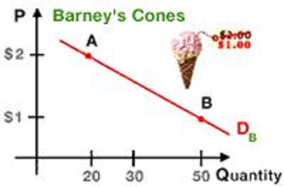
- If the price goes from $2 to $1, what is the price
elasticity of demand?
- Data:
- P1 = $2; Q1 =20;
- P2 = $1; Q2 = 50
- Formula: Ed = | %Qd
/ %P
|
- ME: our textbook calls this the "coefficient of
price elasticity of demand" (Ed)
- ME: see the textbook for the midpoint
formula
- %Qd
= change in quantity / midpoint
- change in quantity = Q2-Q1 = 50 - 20 = 30
- midpoint = halfway between 20 and 50 =
(Q2+Q1)/2 = (50+20)/2 = 70/2 = 35
- %Qd
= change in quantity / midpoint = 30/35 = 6/7
- %P
= change in price / midpoint
- change in Price = P2-P1 = 1-2 = -1
- midpoint = (P2+P1)/2 = (1+2)/2 = 3/2 =
-3/2
- %P
= change in price / midpoint = -1/(3/2) = -2/3
- The video lecture will ask you a
multiple choice question. ANSWER THE QUESTION by selecting A,
B, or C and more of the lecture will follow
- If the price goes from $1 to $2, what is the price
elasticity of demand?
- Data:
- P1 = $1; Q1 = 50
- P2 = $2; Q2 = 20
- you will get the same answer 9/7 or 1 and 2/7;
ERROR: there are two correct answers 9/7 is the same as 1
and 2/7
- using the midpoint formula we estimate the price elasticity
of demand and it does not matter if the price increases or the
price decreases, the elasticity will be the same
- ME: we will always use the midpoint formula
5.1-3 [TW 2.4.3
8:42)] Applying the Concept of Elasticity - 4a
- ME: be sure to read the textbook section: "Interpretations
of Ed" !!
OPTIONAL: Introduction
to Price Elasticity of Demand - Calculating PED Using Data from a
Demand Diagram (econclassroom.com 11:46) -
4a
OPTIONAL: Price
Elasticity of Demand and the Total Revenue Test
(econclassroom.com 13:24) - 4a
5.2-1 [TW 2.4.4
(6:50)] Identifying the Determinants of Elasticity - 4a
- Outline
- What determines the price elasticity of demand?
- Availability of close substitutes
- Time needed to search for a substitute
- Percentage of budget (income) spent on the
good
- ME: the textbook also includes luxuries vs.
necessities
- Review: elastic vs. inelastic
- What determines the price elasticity of demand?
- the price elasticity of demand is:
- the responsiveness of the quantity demanded to changes
in the price of the good
- the % change in quantity demanded that results from a %
change in price
- what determines if the price elasticity of demand for a
good is elastic or inelastic?
- Availability of close substitutes
- many substitutes = more elastic demand
- few substitutes = less elastic
- Time needed to search for a substitute
- more time = more elastic
- less time = less elastic
- ME: students often get this wrong. If the price of gas
increases to $7.00 a gallon today what will happen to the
quantity demanded in the next few weeks? Yes, it will decrease
but by HOW MUCH? Most students say that it would decrease by a
lot, BUT what other alternatives do we have? I think that there
would be only a small decrease in quantity demanded and demand
is less elastic. Now, if we wait six months and then check to
see how consumers responded to that increase in gasoline prices
I think we would see a much bigger response (more elastic)
because they would have had more time to fins substitutes
(check the bus schedule, get a more fuel efficient car, find
friends to share rides with, etc.).
- Percentage of budget (income) spent on the good
- if you spend a small percent of your budget on a product
then demand for that product is less elastic
- if you spend a large percent of your budget on a product
then demand for that product would be more elastic
- ME: the textbook also includes luxuries vs. necessities
- luxuries have a more elastic demand
- necessities have a less elastic demand
- Review: elastic vs. inelastic
- demand for a product is more price elastic if:
- there are many substitutes
- you have lots of time to find substitutes
- if is makes up a large part of your budget
- if it is a luxury
- demand for a good will be less price elastic if:
- it has few close substitutes
- you have little time to find substitutes
- if is makes up a small part of your budget
- you have a necessity
Examining the Effect of an
Excise Tax on an Inelastic Good -- Cigarettes (12:41) - 4a
http://www.econclassroom.com/?p=2771
- An excise tax is either a specific tax or an ad valorem tax
placed on a particular good or service. (ME: we will only look at
a specific excise tax)
- An excise tax is a tax of a specific amount to be paid
on every unit of a product sold. Example: a $2 tax on a pack of
cigarettes
- ME: we won't worry about ad valorem tax, but Illinois does
have a specific excise tax on a gallon of gasoline ($0.19 per
gallon) and an ad valorem excise tax on gasoline (5% of the
price)
- Example: what happens when the government places a $2 tax per
pack on cigarettes?
- we know that taxes decrease supply
- a $2 tax will shift the S=MC curve "upwards" by
$2. At every quantity sold, the cigarette producers
face an additional $2 cost, in the form of the tax
that they must pay to the government
- the amount of the tax is the vertical
distance between the two supply curves
- what happens to the equilibrium price and
quantity as a result of the $2 tax?
- equilibrium quantity will go down; people will
buy fewer packs of cigarettes
- But notice that a $2 tax does NOT increase
the price by $2;
- who pays the tax (bears the burden of the
tax), or how much the price increases, depends on
the price elasticity of demand
- if the demand for cigarettes was perfectly
inelastic (if the demand curve was vertical) then a
$2 tax would cause the price to increase by $2
- but demand is not perfectly inelastic so
customers do not pay the whole amount of the tax
- so if producers did raise the price by the
whole $2 they would make much less profits as
they will lose many customers
- so producers will raise the price by less
than the amount of the tax ($1.20 in the
example) and the producers will pay the rest of
the tax ($0.80) themselves
- Tax burden (or tax incidence) refers
to the amount of the tax paid by producers and
the amount of the tax paid by consumers; ME: our
textbook uses the term "tax
incidence"
- notice that the consumers bear a higher
burden of the tax
- how much tax is collected by the government
is calculated by taking the amount of the tax ($2)
times the quantity sold (25) = $50
- consumers pay $1.2 times 25 = $30 = blue
rectangle
- producers pay $0.80 times 25 = $20 = green
rectangle
- what happen to social welfare (allocative
efficiency)?
- let's assume that there are no externalities
associated with cigarettes, then the original S =
MSC and D = MSB and the original equilibrium
quantity of 30 would maximize society's
satisfaction or it is the allocatively efficient
quantity; this is when the consumer and producer
surplus is maximized
- but with the tax the quantity that consumers
buy is lower; this represents allocative
inefficiency because consumers are buying
less;
- another way to show this is by measuring the
dead weight loss
- consumer surplus decreases (purple
triangle)
- producer surplus also decreases (yellow
triangle)
- government gains $50 in tax revenue
(government surplus?) which can be seen as a
benefit to society (red rectangle = CB +
PB)
- dead weight loss of the tax = loss of social
welfare (satisfaction) caused by the tax (black
triangle)
|
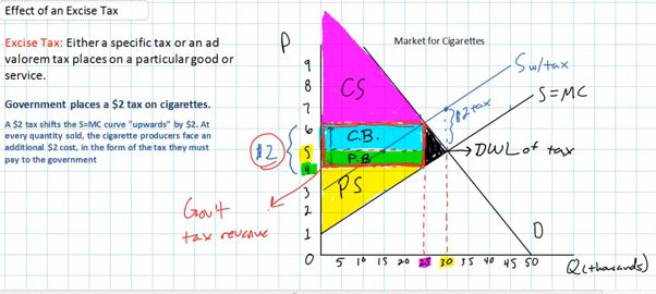
|
- Summary: if we add an excise tax to a product
- supply will decrease causing the price to increase and
the quantity to decrease
- the amount of the tax is the vertical distance between
the two supply curves
- the excise tax is shared between the consumers and
producers; the incidence of the tax depends on price
elasticity of demand
- if the demand is relatively inelastic then the
consumers will pay most of the tax
- if the demand is relatively elastic then the producer
will pay most of the tax
- the amount of tax revenue collected by the government is
the amount of the tax times the new equilibrium quantity
- if the demand is relatively inelastic then the
government will collect more tax revenue
- if the demand is relatively elastic then the
government will collect less tax revenue
- social welfare (allocative efficiency) decreases; there
is a loss of satisfaction to society (dead weight loss ) due
to the excise tax because less will be produced
- if the demand is relatively inelastic then there will
be a small loss of satisfaction to society (only a little
allocative inefficiency)
- if the demand is relatively elastic then there will
be a large loss of satisfaction to society (a lot of
allocative inefficiency)
- we will see in the next video lecture that the amount
of dead weight loss is greater if demand is elastic and
smaller if demand is inelastic
Examining the Effect of an
Excise Tax on an Elastic Good -- Candy Bars (8:08) - 4a
http://www.econclassroom.com/?p=2774
- Review of the previous lecture (excise tax on
cigarettes)
- the excise tax is shared between the consumers and
producers; the incidence of the tax depends on price elasticity
of demand
- if the demand is relatively inelastic (like for cigarettes)
then the consumers will pay most of the tax
- if the demand is relatively elastic (like for candy bars)
then the producer will pay most of the tax
- The demand for candy bars more elastic than the demand for
cigarettes?
- there are lots of substitutes for candy bars and few
substitutes for cigarettes
- cigarettes are also addictive (like a necessity) = less
elastic demand
- the demand curve then will be flatter for candy bars = more
responsive to a change in price (bigger change in Qd when the
price changes)
- Effects of a $2 excise tax on candy bars (elastic demand)
- supply decreases (supply shifts up by $2) causing
the price to increase and the quantity to decrease;
- since the demand is elastic the quantity
demanded (equilibrium quantity) will
decrease A LOT.
- and since the demand is elastic the equilibrium
price paid by consumers will increase only a
little
- the incidence of the tax on consumers
(consumer tax burden) is smaller than the
producer tax burden; the producer will pay most of the
tax
- the amount of tax revenue collected by the
government, tax revenue = $2 excise tax times
quantity, (the blue + green rectangles ) is
small because the quantity sold decreases a
lot
- there is larger dead weight loss (black
triangle), i.e. loss of satisfaction to society
|
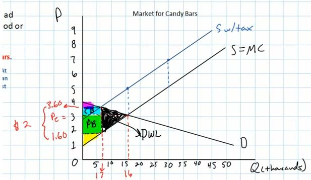
|
- Why tax products with inelastic demand rather than products
with elastic demand?
- if demand is inelastic ( like cigarettes):
- quantity decreases only a little and the price increases
a lot
- incidence of the tax is more on consumers
- government collects more tax revenue
- negative effect on allocative efficiency (dead weight
loss) is less
- if demand is elastic (like candy bars):
- quantity decreases a lot and price increase a
little
- incidence of the tax is more on the producers
- government collects less tax revenue
- negative effect on allocative efficiency (dead weight
loss) is greater
- BUT:
- remember: if there are negative externalities associated
with a product (like cigarettes) then
- too much will be produced
- the government may want to put an excise tax on the
good to decrease the quantity consumed
- BUT (again) if the demand is inelastic, the excise
tax will not have a big effect on the quantity
demanded
MODULE 4b - OTHER TYPES OF ELASTICITY
- PRICE ELASTICITY OF SUPPLY
- CROSS ELASTICITY OF DEMAND
- INCOME ELASTICITY OF DEMAND
Elasticity of Supply (Khan
Academy 9:33) - 4b
http://www.khanacademy.org/finance-economics/microeconomics/v/elasticity-of-supply
CROSS ELASTICITY OF DEMAND
Cross Elasticity of Demand
(Khan Academy 11:20)- 4b
http://www.khanacademy.org/finance-economics/microeconomics/v/cross-elasticity-of-demand
- HOW MUCH does a price change of one good affect the quantity
demanded of another good
- uses the midpoints formula to calculate the percent increase
in price of an airline ticket and the percent change in
quantity
- "CED" = cross elasticity of demand
- cross elasticity of demand = % change in quantity demanded of
one product / % change in price of another product
- if the products are near perfect substitutes then the cross
elasticity of demand will be very high and will approach infinity
(example tickets on different airlines)
- substitutes have + (positive) cross elasticities of
demand (example: Coke and Pepsi)
- complements have - (negative) cross elasticities of
demand (example: e-books and e-reader)
- unrelated products have a cross elasticity of demand
that equals zero
INCOME ELASTICITY OF DEMAND
Income Elasticity of Demand (Gale Pooley 3:14)- 4b
http://www.youtube.com/watch?v=Tct2EmT9iNE
- Edy = coefficient for the income elasticity of demand
- formula = % change in Qd / % change in income
- if Edy < zero, the product is an inferior good
- when incomes increase the quantity bought will
decrease
- example: ramen noodles = inferior good
- if Edy is between zero and one, the product is a normal good
- when incomes increase the quantity bought will
increase
- example: candy bar = normal good
- if Edy > 1, the product is a luxury good
- when incomes increase the quantity bought will increase a
lot
- example: restaurant meal = luxury good
Chapter 6- Consumer Behavior (Module 6a)
MODULE 6a - CONSUMER DECISIONS: UTILITY
MAXIMIZATION
- 6.1-1 Understanding Utility Theory [TW 3.1.1
(4:31)]
- Plotting
MU at the Midpoint (4:50)
www.harpercollege.edu/mhealy/eco211f/screencasts/6aplotatmidpointmu.mp4
- 6.2-1 Optimal Consumer Choice - Finding Consumer Equilibrium
[TW 3.1.2 (4:47)]
- Professor Harmon Calculates the Utility Maximizing Bundle in 5
minutes (YouTube - 02001orh 4:58)
http://www.youtube.com/watch?v=LY1slp1dacA
6.1-1 [TW 3.1.1 (4:31)] Understanding Utility
Theory - 6a
- Outline
- Utility theory
- Measuring total utility (TU) and marginal utility
(MU)
- The law of diminishing marginal utility
- Utility theory
- utility theory explains how households allocate their
budget (spend their money) over a wide array of goods and
services
- ME:
- how much do we buy of each item to maximize our utility
(satisfaction)
- why do we buy what we buy? why do we buy many different
things?
- why don't we just buy the one thing that we like the
best?
- Measuring total utility (TU) and marginal utility (MU)
- economists measure satisfaction (utility) using an
artificial unit called the "Util". A util is an increment of
satisfaction, and artificial construct of utility or
psychological satisfaction
- ME: utils do not exist. We cannot measure satisfaction.
But, economists ASSUME that they can to explain consumer
behavior; to explain why we buy the quantities that we do.
- ME: utility cannot be measured
- ME: utility can be compared. We can say that we like
something more than something else, but we cannot measure the
number of "utils"
- TU is the total satisfaction (number of utils) a consumer
gets from consuming units of a good or service
- MU is the additional satisfaction (number of utils) that a
consumer receives from consuming one additional unit of
a good
- marginal utility diminishes
- ME: MU = TU
/ Qconsumed
- TU is the sum of the MU
- more is better, up to a point, but each additional unit
provides less additional satisfaction than the unit before
- The law of diminishing marginal utility
- after some point consumption is subject to the law of
diminishing marginal utility
- after some point, each additional unit that you consume, in
a set period of time, ceteris paribus, will provide less
additional satisfaction than the unit before
- more of everything is better, but more of one thing in a
given period of time give less and less extra satisfaction and
may give no, or even negative, satisfaction
- ME: we get "sick of it"; this explains why we do not just
eat our favorite food every meal, every day. Even though it is
our favorite food, after a while, we will become sick of it,
i.e. we will get little, or even negative, satisfaction from
additional units
- ME: surprisingly, Professor Tomlinson does not graph TU and
MU. See our textbook and yellow pages for the graphs.
6.2-1 [TW 3.1.2 (4:47)] Optimal Consumer Choice -
Finding Consumer Equilibrium - 6a
- Outline
- How will a household spend its limited income on the
goods and services that provide it with satisfaction?
- The utility maximizing model
- How will a household spend its limited income on the goods and
services that provide it with satisfaction?
- How much will we spend on apples and how much will we spend
on candy bars?
- the utility maximizing rule: to get the most satisfaction
possible, households will spend their income such that the MU
per dollar spent is equal for all items
- MUx/Px = MUy/Py
- To maximize utility, consumers will equalize their marginal
utilities per dollar spent between goods
- The utility maximizing model - an example: candy bars and
apples
- In a two-good model, a consumer continuously reallocates
her income until the marginal utility per dollar spent on one
good is equal to the marginal utility per dollar spent on the
other good
- ME: we can easily expand this model to include more goods
-- to maximize utility consumers will spend their income such
that: MUa/Pa = MUb/Pb = MUc/Pc = MUd/Pd = . . . . .
- An example:
- Given:
- income = $6
- only two items to buy: apples and candy bars
- the price of apples = $1.00
- the price of candy = $ 0.50
- the MU received from different quantities of apples
and different quantities of apples (see table below)
- Question: how many apples and candy bars would be bought
to receive the maximum utility (satisfaction) possible from
the $6 in income?
- consumers will buy an item as long as the MU they
receive per dollar spent on the item is greater than the
MU per dollar that they could bet on a different good;
i.e. buy the item that gives you the most satisfaction
for your money
FIRST you must calculate MU/P for
each product:
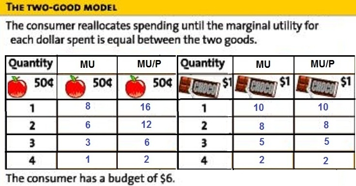
Then: go shopping and buy the item
that gives you the greatest MU for your money (the
highest MU/P):
You will first buy one apple because it give you 16
utils per dollar and the first candy bar gives you only
10 utils per dollar
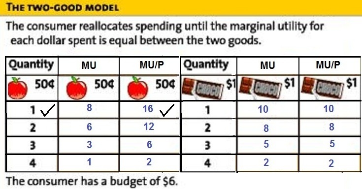
Next you will buy another apple because you get 12
utils per dollar which is more than you would get from
the first candy bar,
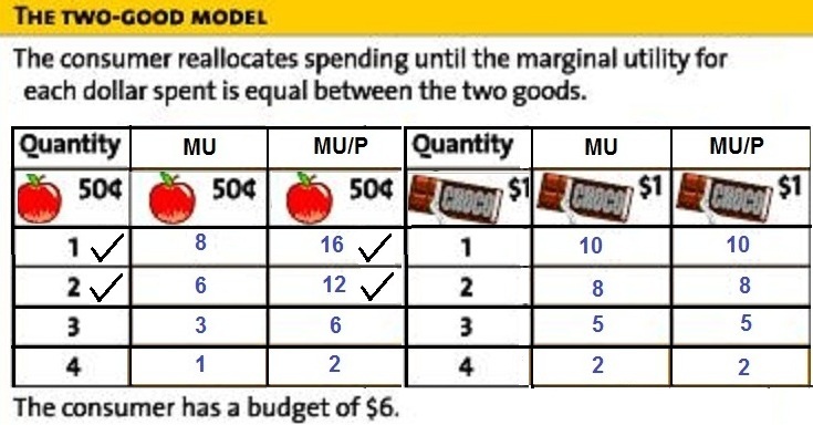
Now you would buy your first candy bar and get 10
utils per dollar (if you bought another apple you would
only get 6 utils per dollar)
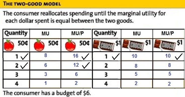
And another candy bar (8 utils per dollar is more than
the 6 utils per dollar that you would get if you bought
another apple)
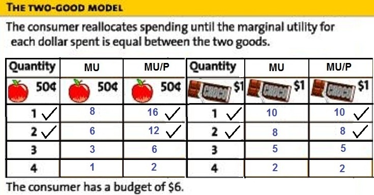
So far you have spent $1 on apples and $2 on candy
bars. You have $6 to spend, so continue to shop. What
would you buy next? Your third apple (6 utils/$ for the
third apple compared to 5 utils/$ for the third candy
bar).
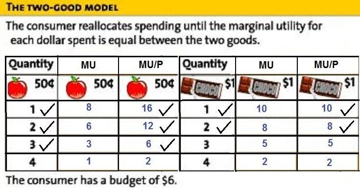
And you continue to shop this way until you have spent
your $6.
ME: This is a strange problem because you end up
buying everything on the table. Be sure to do some of the
"practice exercises" (see link on Blackboard) because in
them you will have to stop shopping when you run out of
money and before you buy everything on the table.
ME: Also, Professor Tomlinson did not have you
calculate the maximum total utility (TU) possible. You
can see from the table below that if you buy 4 apples the
TU you receive is18 utils, and if you buy 4 candy bars
the TU you receive is 25 utils. So, if you spend all of
your $6 income the maximum TU possible is 18 + 25 = 43
utils.
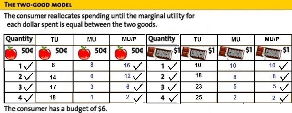
BUT, you may be asking how did we calculate the TU in
the table above? Remember, MU is the extra utility
received from consuming one more. If you add up all of
the marginal utilities, you get the total. For two apples
the TU = 8 + 6 = 14. For three apples the TU is 8 + 6 + 3
= 17.
- ME: be sure to do several practice exercises on these
types of problems.
Professor Harmon Calculates the Utility Maximizing Bundle in 5
mins (YouTube - 02001orh) - 6a
http://www.youtube.com/watch?v=LY1slp1dacA
- ME: You will encounter two different types of utility
maximization problems
- one where you are given the MU (like in the video lecture
above and the "Worked Problem" link above)
- and one where you are given the TU (like in this YouTube
video) and you have to calculate the MU
- Problem:
- Video games cost $12 and spy novels cost $10
- You have $54 to spend
- The TU is given in the table
- Question: What quantity of video games and spy novels should
you buy to maximize your utility and what is the maximum total
utility possible?
- Use the Utility Maximization Rule: always buy the product that
gives you the greatest MU/P (MU per dollar) first, and continue
buying until you have spent all of your money
- First calculate the MU for each product
- Then calculate the MU/P for each product
- Then go shopping buying the product that gives you the
highest MU/P first and continue buying video games and spy
novels until you have spent all $54 or as much as possible.
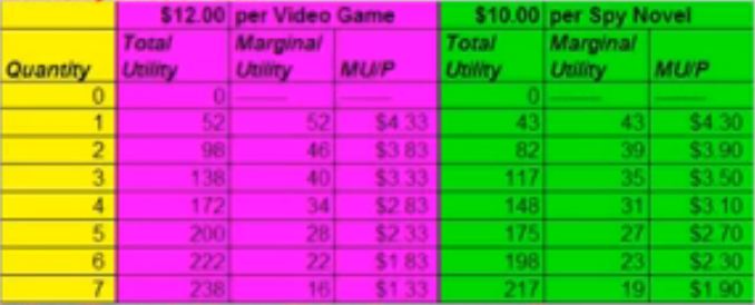
Chapter 7 - The Costs of Production (Modules 7a,
7b, and 7c)
MODULE 7a - ECONOMIC PROFITS AND THE PRODUCTION
FUNCTION
- AN ECONOMIST'S VIEW OF COSTS AND PROFIT
- 7.1-1 Finding Economic Profit [TW 5.1.4
(13:54)]
- PRODUCTION IN THE SHORT RUN
- 7.2-1 Understanding Output, Inputs, and the Short Run
[TW 4.1.1 (8:48)]
- 7.2-2 Explaining the Total Product Curve [TW 4.1.2
(15:57)]
- 7.2-3 Drawing Marginal Product Curves [TW 4.1.3
(7:22)]
- How
to Plot MP at the Midpoint (6:54)
www.harpercollege.edu/mhealy/eco211f/screencasts/7aplotatmidpointmp.mp4
- 7.2-4 Understanding Average Product [TW 4.1.4
10:32)]
AN ECONOMISTS VIEW OF COSTS AND
PROFIT
7.1-1 [TW 5.1.4
(13:54)] Finding Economic and Accounting Profit -7a
- Outline
- economic profit and accounting profit differ from each
other in the way that each defines costs
- calculating economic profits of a firm: compare total
revenues to ALL OPPORTUNITY COSTS of the resources that it
employs
- sunk costs (fixed costs) are prior-occurring costs that
are unrecoverable and should not affect current
decisions
- economic profit is the difference between the revenue that a
firm earns and the sum of the opportunity costs of the all
resources that the firm employs
- ME: economic profit = TR - TC (where TC include all of the
opportunity costs)
- TR = P x Q
- TC includes all of the opportunity costs of the resources
used
- if the total revenue > the sum of the opportunity costs of
the resources the firm is making an economic profit and then the
resources will stay with the firm
- BUT, if the total revenue < the sum of the opportunity
costs of the resources, the firm has economic losses and then the
resources will seek employment elsewhere (go out of business)
- ME: this explains why a zero profit IS GOOD in economics
- Economists vs. accounting profits:
- accounting profit = total revenue - explicit costs
only
- economic profit = total revenue - all of the opportunity
costs
- economic profit = total revenue - (explicit costs +
implicit costs)
- c.o.g.s = cost of goods sold
- accounting profit does not tell us if the
resources in our business are earning as much, or more, than
they could earn in their next best opportunity;
- accounting profit does not tell us if the
resources will stay with our business OR leave for a better
opportunity elsewhere.
- accounting profit does not tell us if our
business will continue to exist.
- because accounting profit does NOT include the
opportunity cost of the resources
- economic profit does take into account what
our resources could earn elsewhere and therefore it tells us if
the resources will stay with us or move elsewhere.
- economic profit does tell us if the resources
will stay with our business OR leave for a better
opportunity elsewhere.
- economic profit does tell us if our business will
continue to exist.
- because it includes the opportunity cost of the
resources (what they could have earned in their next best
alternative)
- economic rent: the amount of payment an economic
resources receives in excess of its next best
alternative
- how much better a resources is doing than in their
next best alternative
- ME: we will call this "economic profit"
- economic profit tells us how much the revenues exceed
the total opportunity costs of all resources employed
- economic profits then are divided among the resources in
the form of economic rents
- if economic profits are negative the business
will end up closing down because the resources would have
better opportunities elsewhere -- even if the accounting
profit is positive; i.e. even though the books look good
according to the accountant, the firm will close down
- ME: this is why a ZERO PROFIT in economics is GOOD;
because a zero economic profit INCLUDES covering all of the
opportunity costs; i.e. you are paying yourself just as much
as you would be paid in your next best alternative,
- what you could make elsewhere is included in the
costs;
- therefore, if TR - TC = zero, you have already
paid yourself and the opportunity costs of all other
resources
- sunk costs are unrecoverable costs incurred in a
previous time period that have no relevance to the current
decisions
- ME: also called "fixed costs"
- ignore sunk costs; they should not affect current
decisions
- to make good decisions you should compare the extra
benefits (MB) and the extra costs (MC); if the MB > MC
then do it, but you should ignore sunk costs
- ME: i.e. do not come to class if you are very ill just
because you already paid the tuition
PRODUCTION IN THE SHORT RUN
7.2-1 [TW 4.1.1
(8:48)] Understanding Output, Inputs, and the Short Run -
7a
- Outline
- How much should a firm produce?
- Definition: Total Output (also called Total
Product)
- Total output in the short run
- Redefining total output
- Total output schedule
- How much should a firm produce?
- Goal: to maximize profits
- WE WILL SPEND THE NEXT 20 OR 30 VIDEO LECTURES ON THIS
TOPIC: How much should a firm produce?
- to answer this we need to took at how a firm makes a
product, i.e. its technology
- then we look at the costs = how much it costs to make a
product
- finally we combine costs with the price a firm can get
for its product
- technology is a catalog (or list) of the things that a firm
knows how to do
- how much output can a firm produce with a given amount
of input
- this is really engineering (technology); what can a firm
do?
- Definition: Total output (also called Total Product)
- total output is the total amount of output that a firm can
produce with a given amount of inputs (resources) and its
technology
- also called Total Product
- ME: sometimes this is called the firm's production
function
- Total output in the short run
- short run is a period of time that is so short that
a company can only change one, or a few, of its inputs
- ME: our textbook introduces short run and long run in
chapter 4 (elasticity chapter);
- in the short run some of the resources are fixed,
i.e. cannot be changed;
- usually the size of the factory (plant) is
fixed;
- in the short run there is not enough time to change
the size of the factory, but you can change the amounts
of variable inputs used
- ME: the video lecture simplifies the short run
definition by saying that only one input is variable
- Tomlinson assumes all resources are fixed except labor;
labor then is the only variable input
- Redefining total output
- total output of the variable input labor is the total
amount of output that a given amount of labor can produce
holding constant technology and all other inputs
- Total output schedule
- how many televisions can be produce in a week with 1
worker, 2 workers, 3 workers, etc, assuming all other inputs
are constant?
- with more workers more televisions can be produced UNLESS
we get too many workers, then the number of televisions
produced will decrease? Why?
- ME: because since we are holding all other inputs
constant, like the size of the factory, the factory is
becoming overcrowded
- a plot of the total output schedule is called the Total
Product Curve
7.2-2 [TW 4.1.2
(15:57)] Explaining the Total Product Curve - 7a
- Outline
- Production Possibilities in the short run
- Graphing the total product curve
- Properties of the total product curve
- The marginal product of labor
- Why does the marginal product change?
- Production Possibilities in the short run
- what a single firm can do in the short run when it adds
more labor assuming all other resources are fixed
- Graphing the total product curve
- always label the axes!
- vertical: the total amount of output or total product
(TP)
- horizontal: the amount of labor (# of workers) or
quantity of variable input
- make the graph
- Properties of the total product curve
- ME: whenever we create a new graph we always
explain its shape!
- S-shape with three different parts
- at first the curve is increasing at an
increasing rate (getting steeper or convex)
- then the curve is still increasing but at a
decreasing rate (getting flatter or concave but
still going up)
- finally the curve reaches a maximum and then if
we add more worker we produce LESS and the curve
goes down
- Why? We will explain the shape of the TP graph
by discussing the marginal product of labor
(MP)
|
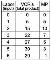
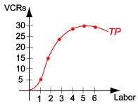
|
- The marginal product of labor
- definition: the change in total output that results from
changing the variable input by one unit; how much more output
we get from each additional worker
- MP = change in TP / change in the quantity of variable
input;
- MP =
TP /
Qinput
- ME: MP is the slope of the TP graph
- MP goes up because TP gets steeper (convex), then MP
goes down because even though TP is still increasing it's
slope is less - getting flatter (concave), finally MP
becomes negative when TP starts to decline, the TP then has
a negative slope
- Why does the marginal product change?
- Why does MP increase at first, reach a maximum and then
declines and finally becomes negative?
- MP increases (TP increases at an increasing rate) at first
because of specialization and teamwork;
- specialization causes increases in productivity through
fewer setup costs
- teamwork: larger groups of workers can use different
techniques that can increase productivity
- MP later decreases (TP increases at a decreasing rate)
because of the problem of congestion -- the factory is
getting crowded; remember the size of the factory is fixed and
it can get crowded. This reduces productivity and the
additional output that results from adding another worker will
decline
- MP eventually becomes negative (TP decreases) because the
factory becomes overcrowded. The factory is so crowded
that the addition of one more worker actually causes output to
decrease.
- ME: this idea of specialization and teamwork, congestion, and
overcrowded, will be used later in this chapter to explain the
shapes of other graphs
7.2-3 [TW 4.1.3
(7:22)] Drawing Marginal Product Curves - 7a
- Outline
- Trying to graph the marginal product
- Intuition about the marginal product curve
- Plotting and connecting
- Change in MP as part of technology
- Convex/concave: a demonic device
- Trying to graph the marginal product
- a graph that describes a firm's technology
- know how the axes are labeled
- MP =
TP /
Qlabor
- Intuition about the marginal product curve
- MP = slope of the TP curve
- MP goes up because TP gets steeper (convex),
- then MP goes down because even though TP is still
increasing it's slope is less - getting flatter
(concave),
- finally MP becomes negative when TP starts to decline -
TP then has a negative slope
- Plotting and connecting
- ME: note when TP is at its peak, MP is zero, (when TP is at
its peak its slope [MP] is zero)
- Change in MP as part of technology
- why does MP increase at first?: specialization and teamwork
possible if more workers are working at the same time together
(see previous lecture)
- why does MP start to decline?: problem of congestion
- why does MP become negative?: overcrowded
- Convex/concave: a demonic device (memory trick)
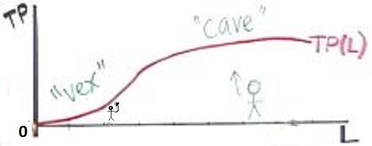
7.2-4 [TW 4.1.4
10:32)] Understanding Average Product - 7a
- Outline
- Marginal Product (MP) vs. Average Product (AP)
- Computing AP
- Graphing AP
- MP and AP together
- MP intersects AP at its maximum point
- Marginal Product (MP) vs. Average Product (AP)
- AP is another measure of productivity
- Using MP, a firm can determine the level of output it has
to produce in order to maximize its profits
- Using AP, a firm can determine whether it will make a
profit or a loss when it is trying to maximize its profits
- Computing AP
- AP is the total output divided by the total quantity of
labor input
- AP = TP/Qlabor or AP = TP/Qinput
- AP is the output per worker
- sometimes called "labor productivity"
- the amount of output that the average worker produces
- Graphing AP
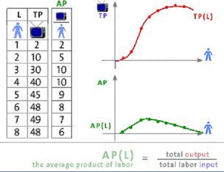
- shape:
- slopes upward than downward (upside down U-shape)
- reaching a maximum (i.e the max. number of televisions per
worker)
- MP and AP together
- when the MP is above the AP, then the AP is rising
- when the MP is below the AP, then the AP is downward
sloping
- the MP crosses the AP when the AP is at its maximum
point
- MP intersects AP at its maximum point
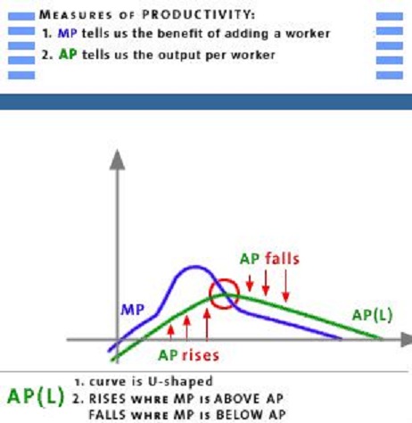
- what happens to your GPA if your "marginal grade point" (GPA
THIS semester) is above your cumulative GPA? It will rise. MP
above AP then AP rises.
- what happens to your GPA if your "marginal grade point" (GPA
THIS semester) is below your cumulative GPA? It will fall. MP
below AP then AP falls
- therefore the MP crosses the AP at the maximum of the AP. This
is the point where labor productivity is at its highest. Know this
because it will be used later.
- JOKE: how can a student leaving one school and going to
another school cause the IQ of both schools to increase? He was
below average at the first school but above average at the other
school.
MODULE 7b -
PRODUCTION COSTS IN THE SHORT RUN
- 7.3-1 Defining Variable Costs [TW 4.2.1 (4:23)]
- 7.3-2 Graphing Variable Costs [TW 4.2.2 (4:57)]
- 7.3-3 Defining Marginal Costs [TW 4.3.1 (6:41)]
- 7.3-4 Deriving the Marginal Cost Curve [4.3.2
(10:59)]
- 7.3-5 Understanding the Mathematical Relationship between
Marginal Cost and Marginal Product [TW 4.3.3 (10:26)]
- 7.3-6 Defining Average Variable Costs [TW 4.4.1
(5:37)]
- 7.3-7 Understanding the Relationship between Marginal Cost and
Average Variable Cost [TW 4.4.3 (7:54)]
- 7.3-8 Defining and Graphing Average Fixed Cost and Average
Total Cost [TW 4.5.1 (6:55)]
- 7.3-9 Calculating Average Total Cost [TW 4.5.2
(4:51)]
- 7.3-10 Putting the Cost Curves Together [TW 4.5.3
(4:51)]
- 7.3-11 Shifts in the Cost Curves [TW 4.6.4
(3:26)]
7.3-1 [TW 4.2.1
(4:23)] Defining Variable Costs - 7b
- Outline
- Definition of variable cost
- Information needed to find variable cost
- Computing variable cost
- The costs of production include:
- variable costs
- fixed costs
- average costs
- marginal costs
- Definition of variable cost
- cost of hiring the variable input needed to produce a
given amount of output
- the total spending on the variable inputs to produce a
given quantity of output
- Information needed to find variable cost
- the amount of labor (variable input) needed to
produce a given amount of output; this is given in the total
product (TP) curve
- the price of the labor or wage rate
- Computing variable cost
- to get the variable cost you multiply the wage rate
times the number of workers
- ME: our textbook calls this the Total Variable Cost (or
TVC); the video lecture calls it simply Variable Costs (VC);
they are the same thing
7.3-2 [TW 4.2.2
(4:57)] Graphing Variable Costs - 7b
- Outline
- Plotting the VC (TVC) curve
- Eliminating inefficient points
- The Maximum total product
- Plotting the VC (TVC) curve
- the VC (TVC) curve shows you how much money must be spent
on labor to produce a given quantity of output
- graph
- horizontal axis: we put the quantity of output
(televisions)
- on the vertical axis we put the costs
- NOTE: if you produce zero televisions then the TVC will
be zero
- Eliminating inefficient points
- no firm will ever hire so many workers so that the output
(TP) begins to decline
- so we won't plot the quantity of television when TP is
declining
- The Maximum total product
- TVC curve becomes vertical since at certain point it does
not matter how much you spend on labor, you can't produce any
more television sets in your given size factory
- again: in our given size factory, the maximum number of
television sets that we can produce is 49 so the VC (or TVC)
curve becomes vertical at that point
- ME: remember our textbook uses TVC and the video lectures
uses VC
- ME: once we draw a new graph we always want to understand
its SHAPE. This will be discussed in a later video lecture
(7.3-4)
7.3-3 [TW 4.3.1
(6:41)] Defining Marginal Costs - 7b
7.3-4 [TW4.3.2
(10:59)] Deriving the Marginal Cost Curve - 7b
7.3-5 [TW 4.3.3
(10:26)] Understanding the Mathematical Relationship between
Marginal Cost and Marginal Product - 7b
- Outline
- Definition: MC and MP
- A mathematical connection
- The inverse relationship between MC and MP
- Mirror images: MC and MP curves
- Maximum MP and minimum MC
- Definition: MC and MP
- MP is the extra output that can be produced when you hire
another worker
- MC is the cost of producing an extra unit of output
- there is an inverse relationship between costs and
productivity
- when productivity increases then cost fall
- when productivity goes down then costs go up
- A mathematical connection
- The inverse relationship between MC and MP
- there is an inverse relationship between costs and
productivity
- when productivity increases then cost fall
- when productivity goes down then costs go up
- Mirror images: MC and MP curves
- note: the horizontal axes in these two graphs are measuring
different things
- Maximum MP and minimum MC
- at the maximum point of the MP curve teamwork and
specialization are maximized and the extra cost of and additional
unit of output (MP)is minimized
- beyond this point, as more is produced, we start to experience
the problem of congestion and productivity (MP falls causing the
extra costs (MC) to increase
- ME: the key to understanding all of this is to understand
(1) specialization and teamwork and (2) the problem of
congestion
7.3-6 [TW 4.4.1
(5:37)] Defining Average Variable Costs (AVC) - 7b
- Outline
- Defining Average Variable Costs (AVC)
- Computing AVC
- AVC and profitability
- Understanding why AVC changes (understanding the shape
of the curve)
- Defining Average Variable Costs (AVC)
- We will use MC in later chapters to help us find the
quantity that firms will produce in order to maximize their
profits
- ME:
- in these later chapters (textbook chapters 8 to 11) we
will use benefit cost analysis (that we studied in chapter 1
of our textbook ) to find that firms will maximize their
profits if they produce all quantities where the marginal
benefits (MB) are greater than the marginal costs (MC) up to
the point where MB=MC. A you should know, when MB=MC we are
making the best decision possible.
- We will use the MC that we calculated in the previous
video lectures and we will combine it with something called
marginal revenue (MR). MR is the extra revenue that a firm
gets when it produces and sells one more unit of output. MR
measures the extra benefits (MB) that a firm gets for
producing one more unit of output.
- So: a firm will maximize its profits if it produces all
quantities where MR>MC up to where MR=MC. This MR=MC
rule is very important. It tells us how much firms will
produce, or WHAT WE GET.
- Then we will look to see if this quantity that we get is
the quantity that WE WANT, or the allocatively efficient
quantity. We will do this in chapters 9, 10, and 11 of our
textbook. This is the ultimate goal: to see if profit
maximizing firms will produce the efficient quantity that
society wants.
- we use MC (and MR) to see what quantity of output firms
will produce (how much to produce)
- we use average costs to see if the firms are making any
profit or not at this level of output (are we making a
profit?)
- Definition of AVC: the cost of variable resources (like
labor) per unit of output produced
- Computing Average Variable Costs (AVC)
- AVC = VC/TP
- ME: our textbook uses the formula: AVC = TVC /
Qproduced
- variable costs per unit produced or labor costs per unit
produced
- AVC is the total amount spent on variable costs like labor
divided by the quantity of output produced
- AVC and profitability
- if AVC is greater than the price of the product then firms
will by making a loss
- if AVC is less than the price of the product then the firm
is making enough to cover all of the labor costs and they will
also have some left over to pay some of the fixed costs of
production (like rent on the factory, etc.)
- ME: AVC will help us later to see if we should continue to
produce or not in the short run
- AVC is a guide to help us begin to understand whether
producing a certain level of output could be profitable
- Understanding why AVC changes (understanding the shape of the
curve)
- why does he AVC curve decrease at first, then increase, as
more output is produced?
- it depends on productivity
- if your workers are more productive then fewer will be
needed to produce the product and the average costs will be
lower
- if our workers are less productive than more workers
will be need to produce a given level of output and the
average costs (costs per unit) will be greater
- ME: remember --
- worker productivity increases because of specialization
and teamwork so average costs decrease
- worker productivity decreases because of the problem of
congestion so average variable costs will increase
7.3-7 [TW 4.4.3
(7:54)] Understanding the Relationship between Marginal Cost and
Average Variable Cost - 7b
- Outline
- Marginals and Averages
- Marginal Cost: a review
- Putting AVC and MC together
- MP and AP with MC and AVC
- Marginals and Averages
- marginals and averages always have the same relationship
- if marginal is above average, then the average is going
up
- when marginal is below average, the average is going
down
- and marginal will cross the average at the highest point
of the average
- we saw this when we graphed the MP and AP curves
- we discussed this when we said:
- if your "marginal grade point" (grade point average this
semester only) is above your overall GPA, then your GPA will
increase
- if your marginal grade point this semester is below your
GPA, then your GPA will decrease
- we will see this same relationship with MC and AVC
- Marginal Cost: a review
- MC is the slope of the TVC curve at any point
- at the point of inflection on the TVC curve the MC will be
at its lowest point
- at first the slope of the TVC curve is decreasing (getting
flatter) so the MC is decreasing; then after the inflection
point, the slope of the TVC curve increases (gets steeper) so
MC increases
- Putting AVC and MC together
- we know that AVC will reach its minimum point when it
crosses the MC curve
- if MC is below AVC then AVC will be pulled down
- if MC is above AVC then AVC will be pulled up
- ME: we could also plot AVC curve by plotting the numbers in
the table that we calculated in the previous video lecture
- NOT REQUIRED: How did we know WHERE AVC crosses the MC: or
WHERE AVC is at its lowest point?
- AVC is equal to the slope of a line that runs from the
origin to a point on the VC curve
- the slope of that line = rise/run = VC/Q = AVC
- AVC then will be at its minimum when that slope of this
line is the lowest; i.e. when the slope of a line from the
origin that touches the TVC curve is the flattest
- MP and AP with MC and AVC
- a upside down mirror image of the MC curve is the MP curve;
MC is reciprocally related to the MP
- an upside mirror image of the AVC curve is the AP curve;
AVC is reciprocally related to the AP curve
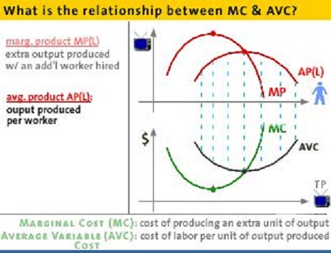
- the more workers it take to produce a unit of output the
higher the costs AND the more workers it takes to produce a
unit of output the lower the productivity and therefore it will
take more workers
- costs and productivity are reciprocally related
7.3-8 [TW 4.5.1
(6:55)] Defining and Graphing Average Fixed Cost and Average
Total Cost - 7b
- Outline
- Costs in the short run
- Defining Fixed Cost
- Calculating fixed costs per unit of output
(AFC)
- Graphing AFC
- AFC + AVC = ATC
- Costs in the short run
- the short run is a period of time that is so short that at
least one input (resource) is fixed; usually we assume that the
size of the factory (or plant) is fixed in the short run
- the costs of production then include the variable costs and
the fixed costs
- Defining Fixed Cost (FC = TFC)
- fixed costs are the costs of fixed inputs (resources)
- the fixed costs are costs that do not change even if we
produce more
- ME: fixed costs are costs that we have to pay even if
nothing is produced
- ME: the video lecture uses "FC" for total fixed costs
whereas our textbook uses TFC for total fixed costs
- TFC stay the same at every level of output (even zero)
- to keep things simple the video lecture assumes at ALL
costs are fixed except labor in the short run
- ME: therefore if we graph TFC it would be a horizontal
line
- Calculating fixed costs per unit of output (AFC)
- fixed costs per unit = average fixed costs = AFC
- AFC = TFC/Qproduced = TFC/TP = FC/TP
- AFC is the fixed costs per unit of output; or spreading the
fixed costs even among hate quantity of output produced
- AFC then declines as more is produced; as the quantity
produced increases the AFC gets smaller and smaller and
smaller
- ME: our textbook authors simplify the calculation of AFC
(and AVC and ATC) by using a table of data where the quantity
produced increases by 1;
- Graphing AFC
- as the quantity produced increases the AFC gets smaller and
smaller and smaller
- graph is called a rectangular hyperbola in geometry
- ME: I often do not include the AFC graph on my graphs
because as we will see below you can easily calculate AFC = ATC
- AVC; this way I have few lines on my graphs to keep it
looking simple, but we can still calculate AFC by a simple
subtraction
- AFC + AVC = ATC
- if we add the AFC to the AVC we get the total cost per unit
of output = ATC = average total costs
- ATC = AVC + AFC
- ME: The video lecture is a little sloppy when they graphed
the ATC; The ATC and the AVC curves should be getting closer
and closer together as the quantity increases; this is because
the difference between them is the AFC which keeps getting
smaller and smaller as more is produced
7.3-9 [TW 4.5.2
(4:51)] Calculating Average Total Cost - 7b
- Outline
- Total Cost and profitability
- Defining Average Total Cost (ATC)
- Calculating ATC: two methods
- ATC in short
- Total Cost and profitability
- profits = total revenue - total costs = TR - TC
- profit per unit of output = price - ATC
- Defining Average Total Cost (ATC)
- ATC is the total cost of producing a certain quantity
divided by the quantity produced
- the the total cost PER UNIT of output
- ATC = TFC / Qproduced
- total costs of production include the total fixed costs
plus the total variable costs
- TC = TFC + TVC
- in the video lecture the TFC = $10,000 and the TVC is
the number of workers times the wage rate; wage rate is
$1000;
- with one worker the TVC = 1 x $100 = $1000; total
cost then is TFC + TVC = $10,000 + $1,000 = $11,000
- with two workers the TVC = 2 x $100 = $2000; total
cost then is TFC + TVC = $10,000 + $2,000 = $12,000
- ATC = TC/Qproduced = TC/TP
- Calculating ATC: two methods
- ATC = TC/Qproduced = TC/TP
- ATC = AFC + AVC
- ME: Professor Tomlinson in the video lectures always runs
through the algebraic steps in his calculation; you should
remember from junior high math class that you if you do
something to one side of an equation then you must do the same
thing to the other side
- ME: where professor Tomlinson uses TP, our textbook usually
uses the quantity produced (Qproduced) or often just "Q".
- ATC in short
- ATC = TC/Q or TC/TP
- ATC = AFC + AVC
7.3-10 [TW 4.5.3
(4:51)] Putting the Cost Curves Together - 7b
- Outline
- Reviewing AVC: cost and productivity
- Components of ATC
- What to remember about ATC and AVC
- The Marginal Cost curve (MC)
- Profit maximizing levels of output
- Reviewing AVC: cost and productivity
- ME: we will be using the following curves a lot: ATC, AVC,
and MC !!
- the AVC curve is the mirror image of the AP curve and
displays the changed in productivity as we add more workers and
produce more
- specialization and teamwork: productivity increases and
costs fall
- problem of congestion" productivity decreases and costs
rise
- Components of ATC
- ATC = AVC + AFC
- the shape of the ATC (remember: we must try to understand
the shape of all of our graphs)
- ATC falls at first as production increases because
- you are able to spread the fixed costs out over a
greater range of output; ATC falls at first because AFC
fall; Tomlinson sometimes uses the term "overhead
spreading" for this concept
- increasing productivity due to specialization and
teamwork means that it take fewer workers on average to
produce a unit of output
- then ATC increases as production increases even though
AFC continues to fall because of the problem of congestion
which decreases labor productivity
- the minimum point of ATC is at a higher level of output
than the minimum point of AVC
- What to remember about ATC and AVC
- the distance between the ATC and the AVC is the
AFC
- the ATC curve and the AVC curve get closer and closer
together as the quantity produced increases
- because the AFC is decreasing as output increases
- The Marginal Cost curve (MC)
- when drawing the MC curve be sure that it passes
through the LOWEST POINTS of the AVC and the ATC curves
- because when the marginal is below the average it pulls the
average down and when the marginal is above the average it
pulls the average up
- remember that the shape of the MC curve is also because of
the changing productivity of labor caused by specialization and
teamwork and by the problem of congestion
- Profit maximizing levels of output
- We will be using these three curves (ATC, AVC, and
MC) to show the profit maximizing level of output that
businesses will produce
- these three curves summarize the firm's productivity and
the costs of the resources that the firm uses
- How do we find the profit maximizing level of output in the
short run?
- The video lecture will ask you a
multiple choice question. ANSWER THE QUESTION by selecting
A, B, or C and more of the lecture will follow
- This is a trick question
- because we have not yet discussed anything about the
revenue the we earn when we sell our product, all we have is
information about costs; we do not have any information
about at what price we can sell our output
- ME: the profit maximizing level of output will be that
quantity where MR=MC
- ME: in later chapters (textbook chapters 8-11) we will use
benefit cost analysis (that we studied in chapter 1 of our
textbook ) to find that firms will maximize their profits if
they produce all quantities where the marginal benefits (MB)
are greater than the marginal costs (MC) up to the point where
MB=MC. A you should know, when MB=MC we are making the best
decision possible.
- We will use the MC that we calculated in the previous
video lectures and we will combine it with something called
marginal revenue (MR). MR is the extra revenue that a firm
gets when it produces and sells one more unit of output. MR
measures the extra benefits (MB) that a firm gets for
producing one more unit of output.
- So: a firm will maximize its profits if it produces all
quantities where MR>MC up to where MR=MC. This MR=MC
rule is very important. It tells us how much firms will
produce, or WHAT WE GET.
- Then we will look to see if this quantity that we get is
the quantity that WE WANT, or the allocatively efficient
quantity. We will do this in chapters 9, 10, and 11 of our
textbook. This is the ultimate goal: to see if profit
maximizing firms will produce the efficient quantity that
society wants.
- we use MC (and MR) to see what quantity of output firms
will produce (how much to produce)
- ME: the video lectures says that we will discuss REVENUES
NEXT, but actually we will not get to revenues until unit three
(chapter 8).
7.3-11 [TW 4.6.4
(3:26)] Shifts in the Cost Curves - 7b
- Outline
- Shifts in the cost curves
- A change in the price of labor: a change in variable
costs
- A change in the price of capital: a change in fixed
costs
- A change in technology
- Shifts in the cost curves
- Review
- MC is upward sloping because of the diminishing marginal
product of labor
- the MC crosses the ATC and the AVC curves at their
minimum points
- the vertical distance between the AT and the AVC
measures the AFC
- cost curves shift when you change a variables that were
held constant while drawing the curves
- input prices
- price of labor
- price of capital
- technology
- A change in the price of labor: a change in variable costs
- ME: labor is a variable resource
- an increase in the price of a variable resource like labor
results in upward shifts of the MC, ATC and the AVC
- ME: recall that we will be using the profit maximizing
rule: MR=MC, to find the quantity that firms will produce. If
the price of a variable input increases, this will shift up the
MC and reduce the profit maximizing quantity
- since there has been no change in the fixed costs, the
distance between the new ATC and AVC does not change
- A change in the price of capital: a change in fixed costs
- capital in our example is a fixed cost (ME: capital isn't
always a fixed cost)
- an increase in the price of a fixed input results in the
upward shift of only the ATC
- the ATC will still cross MC at the minimum point of the
ATC
- and the distanced between ATC and AVC will still get
smaller and small are the quantity of the product
increases
- note that the variable costs did not change so the AVC and
the MC curves do not shift
- since fixed costs increases, the distance between the ATC
and the AVC, which measures the fixed costs, gets wider
- ME: recall that we will be using the profit maximizing
rule: MR=MC, to find the quantity that firms will produce. If
the price of a fixed input increases, this will shift up the
ATC only. It will not change MC (the extra costs of producing
one more unit of output, so it will not change the
profit maximizing level of output. Recall that in benefit-cost
analysis we "ignore fixed costs"
- A change in technology
- an improvement in technology generally results in a
downward shift of the cost curves depending on the nature of
the technological change
- improved technology will result in higher productivity so
it will take few inputs to produce our product which will lower
the costs of production
- ME: recall that we will be using the profit maximizing
rule: MR=MC, to find the quantity that firms will produce. If
technology improves, this will shift the MC curve down (lower
coasts) and increase the profit maximizing quantity
MODULE 7c -
PRODUCTION COSTS IN THE LONG RUN
- 7,4-1 Defining the Long Run [TW4.6.1 (5:55)]
- 7.4-2 Determining the Firm's Return to Scale [TW 4.6.2
(9:01)]
- 7.4-3 Understanding the Short Run and Long Run Average Cost
Curves [TW 4.6.3 (15:06)]
7,4-1 [TW4.6.1
(5:55)] Defining the Long Run - 7c
- Outline
- The long run defined
- Reviewing the short run
- What the firm decides in the long run
- Technique and scale
- The long run defined
- ME: in chapter 9-11 we will use the long run costs curves
to see if different types of firms achieve efficiency (both
allocative and productive)
- the long run is a period of time in which all inputs become
variable so it has not fixed resources and therefore no fixed
costs
- ME: note -- you still have the capital resources like
the factory, but now there is enough time to change the size
of the factory so the plant size has become a variable
resource
- in the long run the firm must consider two thing:
- the technique it will use
- the size, or scale, of the factory
- Reviewing the short run
- a firm aways maximizes it profits where MR=MC (or P=MC in
competitive industries)
- ME: I know that Tomlinson said that profits are
maximized where P = MC, but we will see later that this is
only true in competitive industries (chapter 8 and 9 in our
textbook)
- ME: also, I know that we have not yet seen a video
lecture where he discusses how to maximize profits. i am not
sure why he is calling that a "review"
- in the short run some resources, like the size of the
factory, is fixed so there are fixed costs
- in the short run the only way to increase output is to add
more variable resources like the number of workers
- the problem of congestion occurs only in the short run
which causes productivity to fall and MC to go up
- What the firm decides in the long run
- there are two important decisions that are independent of
each other in the long run, but are related to each other in
the short run
- (1) the choice of the technique of production, or how a
firm combines its inputs, or the ration of labor to capital
- the technique can be capital intensive where a
lot of capital is combined with few workers
- or it can be labor intensive where a lot of
labor is combined with only a little capital
- (2) how big the operation will be, or the
scale
- in the short run these two decision are linked together
- if a firm wants to expand its output (produce more) then
it will add more labor (variable resource),
- THIS will change the technique to one that is more labor
intensive
- Technique and scale
- two independent decisions in the long run
- cost minimizing technique (the ratio of worker to
capital)
- the scale of operation that will maximize profits
7.4-2 [TW 4.6.2
(9:01)] Determining the Firm's Return to Scale - 7c
- Outline
- Considering optimal scale
- Defining scale
- Constant returns to scale
- Increasing returns to scale
- Decreasing returns to scale
- Considering optimal scale
- ME: Tomlinson says that we discussed the choice of
selecting the cost minimizing technique in previous lectures.
Although, we introduced the issue in the previous lecture, I
don't think we got to see the lectures that discussed this.
don't worry
- here we will discuss what is the right size of operation
for maximizing profits?
- review: in the short run a firm must change its technique
AND its scale at the same time. To produce more (increase its
scale) it will add more labor to its given fixed inputs and
this will change the technique (makes it more labor
intensive)
- review: in the long the scale of operation can be decided
independently of the ratio of workers to capital
- since in the long run the scale of an operation can be
decided independently of the ratio of workers to capital
(technique) the long run costs are always lower than the short
run costs; the firm has more flexibility
- Defining scale
- scale is said to increase if it has a proportional increase
in all of its inputs
- example of an increase in scale:
- one worker and one tool
- two workers and two tools
- three workers and three tools
- etc.
- to have an increase in scale it is required that all
inputs increase by the same proportion
- if we just increase labor and hold the amount of capital
constant then that is not an increase in scale ME: by
definition this would be a change in technique
- ME: Note that Tomlinson appears to be inconsistent in
the use of this definition. At the beginning of this lecture
he said something like, "in the short run a firm must change
its technique AND its scale at the same time", but later he
says something like, "if we just increase labor and hold the
amount of capital constant then that is not an increase in
scale". Well, this can be a bit confusing. I think what he
means is IF we change the proportion of capital to labor
(example: instead of one worker and one tool we do two
workers and one tool) then we call this a change in
technique, not a change in scale. Don't worry too much about
it.
- How does a firm's productivity (and therefore costs) change
as we change the scale of operation?
- to answer this question we need to understand another
concept: "economies of scale"
- as we change scale, what happens to output?
- if we go FROM 1 worker and one tool TO two workers and
two tools, what happens to output?
- Constant returns to scale
- if doubling both of our inputs (workers and tools) causes
output to double as well then we say that there are constant
returns to scale
- definition: a technology where increasing all inputs by a
given proportion will increase output by the same
proportion
- constant returns to scale seems reasonable due to the
concept of replication
- Increasing returns to scale
- if doubling both of our inputs (workers and tools) causes
output to MORE THAN DOUBLE then we say that there are
increasing returns to scale
- definition: a technology where increasing all inputs by a
given proportion will increase output by the a greater
proportion
- why? teamwork and specialization
- Decreasing returns to scale
- if doubling both of our inputs (workers and tools) causes
output to increase, by less than double the amount then we say
that there are decreasing returns to scale
- definition: a technology where increasing all inputs by a
given proportion will increase output by the a smaller
proportion
- what would cause decreasing returns to scale?
- management problems may occur in a large organization
- influence activities are efforts on the part
of workers to influence the organization to their
advantage
- ME: see chapter 7 of our textbook for a better and more
detailed explanation of increasing returns to scale and
decreasing returns to scale
7.4-3 [TW 4.6.3 (15:06)] Understanding the Short Run
and Long Run Average Cost Curves - 7c
- Outline
- Reviewing the long and short run
- The long run average cost curve
- Costs in the long run
- Cost minimizing point
- Point of efficient scale
- Reviewing the long and short run
- long run: all inputs are variable (we can change all
resources including the size of the factory)
- short run: some inputs are fixed (we cannot change the size
of our factory)
- The long run average cost curve
- U-shape
- downward sloping part represents increasing returns to
scale
- average costs (costs per unit) costs go down as we
increase the scale
- ME: our textbook uses the term "economies of
scale"
- the bottom represents constant returns to scale
- the upward sloping part represents decreasing returns to
scale
- average costs increase as we increase the scale
- ME: out textbook calls this "diseconomies of
scale"
- Costs in the long run
- when Tomlinson says "suppose that we freeze capital at a
particular level of output and allow the firms to change only
labor" he is talking about a short run cost curve with a given
size factory (amount of capital)
- why does it cost a firm more to change its output in the
short run than it does in the long run?
- The video lecture will ask you a
multiple choice question. ANSWER THE QUESTION by selecting
A, B, or C and more of the lecture will follow
- the firm has more options: they can change the technique
and/or the scale independently
- in the short run all they can do is change the number of
workers
- so the short run cost curves lie above the LRAC except at
one point where the firms are using the cost minimizing
technique
- to change output in the short run you can hire more labor
and move along the short run ATC curve but now you are above
the LRAC curve
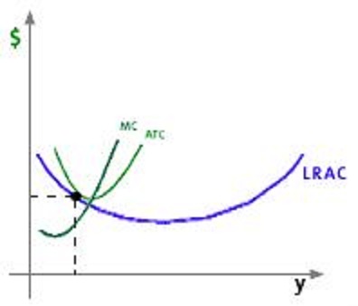
- Cost minimizing point
- what if we freeze capital at the level of output
corresponding to the lowest point on the LRAC curve? (ME"
another way of saying this is" what if we chose a factory size
that corresponds to the level of output at the lowest point on
the LRAC curve?)
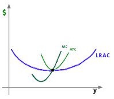
- Summary:
- REPEAT: in the short run the ATC will be higher than the
LRAC because in the long run there is more flexibility (more
options) of finding the cost minimizing technique
- The LRAC curve is an "envelope" of all the possible short
run ATC curves
- only at the very bottom of he LRAC curve are the two
curves tangent at their lowest points
- ME: it seems like we are missing a video lecture because
Tomlinson says, "we have looked at three extreme cases of the LRAC
curve", but we didn't. See your textbook and study the three cases
seen in the figure below
- constant returns to scale over a wide range of output (or
constant returns to scale)
- economies of scale over a wide range of output (or
increasing returns to scale)
- diseconomies set in at a low level of output (or decreasing
returns to scale)
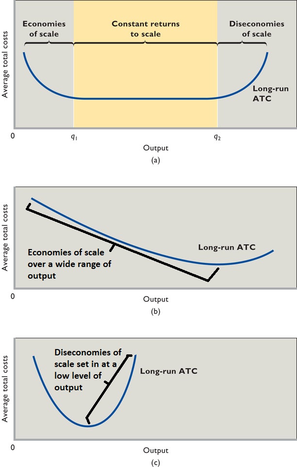
- Point of efficient scale
- U-shape LRAC
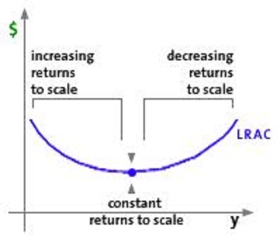
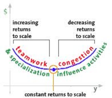
- the point at the bottom of the LRAC curve is called Point
of efficient scale
- the size where the long run average costs are minimized;
where ether is a very short area of constant returns to
scale on the figure above.
- (ME: our textbook discusses a similar concept called the
"minimum efficient scale" which is the minimum level of
output where the LRAC curve is minimized; quantity Q1 on the
figure below
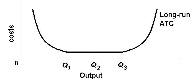
UNIT 3
Chapters 8 and 9 - Pure Competition (Modules 8/9a
and 8/9b)
MODULE 8/9a - PURE COMPETITION: CHARACTERISTICS
AND SHORT RUN EQUILIBRIUM
- MARKET STRUCTURE
- 10.1-1 Understanding Market Structure [TW 5.1.3
(10:55)]
- WHAT IS A PERFECTLY COMPETITIVE MARKET? (PURE COMPETITION)
- 8.1-1 Understanding the Role of Price [TW 5.1.2
(3:43)]
- 8.2-1 Calculating Total Revenue [TW 5.1.1
(3:36)]
- PURE COMPETITION - SHORT RUN PROFIT MAXIMIZATION
- 8.3-1 Finding the Firm's Profit Maximizing Output Level
[TW 5.2.1 (14:24)]
- 8.3-2 Proving the Profit Maximizing Rule [TW 5.2.2
(4:20)]
- 8.3-3 Calculating Profit [TW 5.2.3 (12:26)]
- 8.3-4 Calculating Loss [TW 5.2.4 (9:13)]
- 8.4-1 Finding the Firm's Shut-Down Point [TW5.2.5
(8:35)]
- PURE COMPETITION - SHORT AND LONG RUN MARKET SUPPLY
- 8.5-1 Deriving the Short-Run Market Supply [TW 5.3.1
(20:44)]
- 8.7-1 Deriving the Long-Run Market Supply Curve [TW
5.3.4 (9:13)]
MARKET STRUCTURE
10.1-1 [TW 5.1.3
(10:55)] Understanding Market Structure - 8/9a
- Outline
- The Relevance of Market Structure
- Perfect Competition
- Monopoly
- Monopolistic Competition
- Oligopoly
- The Relevance of Market Structure
- the structure of a market determines whether a firm can
exercise market power (set its own price) or make a profit in
the long run
- Perfect Competition
- large number of small firms
- producing identical products
- therefore each firm has no market power (the-y are price
takers)
- the demand for an individual firm is therefore horizontal
at the market price (perfectly elastic)
- no barriers to entry; therefore if there are short run
profits then new firms will enter the industry until economic
profits equal zero (called a "normal profit) until
- ME: an extreme market with few real-world examples, BUT if
it did exist it would be best for society, i.e. in the long run
competitive markets achieve both allocative and productive
efficiency
- Monopoly
- another extreme market with few real-world examples
- only a single large producer serving the whole market
- therefore they can set there own prices (they have market
power)
- the monopolist's demand curve is downward sloping because
it IS the market demand curve since they are the only producer
in the market
- monopolies arise because of very good barriers to entry
(ME: our textbook says that for a pure monopoly entry is
blocked)
- ME: in the long run monopolies are both allocatively and
productively INEFFICIENT
- Monopolistic Competition
- a hybrid of monopoly and competition (characteristics of
both)
- a large number of firms (like pure competition)
- producing differentiated products; each making their
products a little different than their competitors (each is
like a little monopoly)
- this gives the monopolistically competitive firms a little
market power; some can charge high prices if consumers prefer
their product over others
- ME: therefore the demand curve for each firm is downward
sloping but very elastic since for consumers there are many
other substitute products available
- the market demand curve is downward sloping because it
is the summation of the individual demand curves of all
firms in the industry
- no barriers to entry (ME: our textbook says that there are
some barriers, but they are low and easily overcome)
- Oligopoly
- few firms
- may produce identical (standardized) or differentiated
products
- have a lot of market power
- BUT, since there are just a few producers they carefully
watch what their rivals are doing, called mutual
interdependence
- there are significant barriers to entry
- what does the demand curve look like for oligopolies:
- economists disagree
- the kinked demand curve is a popular theory
- assume:
- that rivals ignore if one firm raises its price
because they will probably get more customers
- but rivals will match the price change if one
firms decides to lower its price to try to keep their
customers
- ME: result: the demand curve will be kinked
- it will be more elastic (flatter) above the
original price because if one firm raises its price
AND all of its competitors do not, then the firm will
lose A LOT of customers
- the demand will be less elastic (steeper) below
the original price because if one firm decides to
lower its price all of its competitors will ALSO lower
their prices and each would get only A FEW new
customers
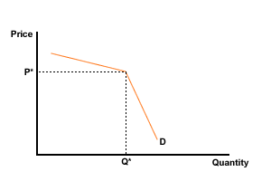
- Summary - ME: the textbook has a more detailed table in
chapter 8 -- Study it!
WHAT IS A PERFECTLY COMPETITIVE
MARKET? (PURE COMPETITION)
8.1-1 [TW 5.1.2
(3:43)] Understanding the Role of Price - 8/9a
- Outline
- Market Power and Price
- a firm with market power can set its own
price
- firms with market power are usually large relative to
market size
- Perfect Competition
- a large number of sellers
- selling identical goods (standardized or
homogeneous)
- no barriers to entry
- Firm and Market demand in Perfect Competition
- an individual firm's demand curve is horizontal
(perfectly elastic) at the market price
- the firm is a price taker
- total revenue equals price times quantity: TR = P x Q or TR =
P x Y
- market power determines the price a firm is able to charge for
its product
- market power is a firm's ability to set the price of
its product
- if a firm can raise the price of its product without losing
all of its customers to a competitor
- if a firm can lower the price of its product without
attracting the entire market
- what determines if a firm has market power?
- how large a firm is compared to the size of the market
- perfect competition:
- large number firms
- each firm is small compared to the market
- firms sell identical goods
- there are no barriers to entry.
- they are price takers = no market power
- each firms only produces a very small share of total market
demand
- identical product - therefore customers do not care who
they buy from
- the supply and demand in the market sets the price for all
of the firms (they are price takers)
- and the demand for a single firm is horizontal
(perfectly elastic)
8.2-1 [TW 5.1.1
(3:36)] Calculating Total Revenue - 8/9a
- Outline
- computing Total Revenue
- plotting the total revenue curve
- slope of the total revenue curve
- total revenue equals price times quantity: TR = P x Q or TR =
P x Y
- ME: total revenue is how much the firm puts in its cash
register
- plotting the TR curve = a straight upward sloping line
- the slope of the TR curve is equal to the price of the product
(the slope of the TR curve is 500 for televisions in a perfectly
competitive market selling television sets)
- ME: Is the market for television sets perfectly competitive?
NO!
- there are not very many companies producing television
sets
- most television producers mare quite large companies
- all television sets are not identical
- there are barriers to entry -- what would it cost for you
to start a company to produce an sell televisions?
- television producers do have market power
- if one producer raises its price a little it does not
lose ALL of its customers
- If one producer lowers its price a little it does not
gain ALL television buyers
PURE COMPETITION - SHORT RUN
PROFIT MAXIMIZATION
8.3-1 [TW 5.2.1
(14:24)] Finding the Firm's Profit Maximizing Output Level -
8/9a
- Outline
- strategies for profit maximization
- understanding the competitive firm
- marginal cost, price, and profit
- marginal revenue and marginal cost
- intuiting the maximum profit
- GOAL: maximizing profits
- RULE: produce another television set as long as it adds more
to revenues than it adds to costs
- never produce another television set if it adds more to
your costs than to your revenues - this would cause profits to
decline
- in pure competition (a competitive firms) should continue
to produce as long as the price it gets (P) is greater than its
marginal costs (MC)
- if the marginal cost is less than its price then produce
more to add to your profits
- maximum profit occurs when P = MC
- ME:
- this rule (P = MC) only works for perfectly competitive
firms
- ALL firms (including competitive firms) maximize their
profits when MR = MC
- we will study this in the next chapters, but the MR=MC
rule to find the quantity where a firm receives the maximum
profit does work for pure competition as well
- the TC and TR graph
- why is the TR curve a straight line?
- why does the TC curve have the "backwards S"
shape"?
- the MR and MC graph ("double decker" graph)
- MR
- definition: the extra revenue that a firm gets when
it produces and sells one more unit
- formula: change in TR / change in Q
- also: MR is equal to the slope of the TR curve
- graph: in pure competition (only) the MR curve is a
straight horizontal line that is equal to the product
price
- MR = P = $500; MR = Price ONLY IN PURE
COMPETITION
- in later chapters MR DOES NOT equal price
- MC
- definition: the extra cost of producing one
additional unit of output
- formula: the change in TC / change in Q
- also: MC is equal to the slope of the TC curve
- graph:
- at first goes down then reaches a minimum (where
the inflection point is on the TC curve)
- crosses the P (or demand) curve at the profit
profit maximizing level of output (Y* or Qprof
max)
- ME: I do not care too much about the Y dagger
quantity
- the profit maximizing level of output using the TR
and TC graph
- Y* in the video lectures; ME: I like to simply use "Q"
or "Q prof max"
- output level ( or quantity) where P = MC
- ME: where the gap between the TC and TC curves is the
greatest (with TR being greater than TC)
- Tomlinson: where the slope of TC = slope of TR
- the profit maximizing level of output using the P
and MC graph
- Y*
- where P = MC (or MR = MC)
- at a quantity greater than Y* (Qprof max) the MC is
greater than price and therefore your profits are declining;
it is costing you more for each additional unit produced
(MC) than you are getting (P = MR)
- at a quantity less than Y* the MC (extra cost of
producing one more) is less than the price (or MR) that you
get, so if you produce more you will be getting more than it
costs you and your profits will increase
- Ydagger is where your profits are the lowest; any point
less or more than Y dagger will be better for the firm
- P=MC is the rule for maximizing profits for a purely
competitive firm as long as the MC curve is increasing
8.3-2 [TW 5.2.2
(4:20)] Proving the Profit Maximizing Rule (Pure Competition) -
8/9a
- Outline
- the rule for profit maximization
- proving it with real numbers
- discerning whether the max profit point will yield a
positive profit
- ME: the lecture begins with the table below. Here he is using
the production function from lectures 7.2-1 and 7.2-2 where "L" is
the quantity of labor in our factory (number of workers) and TP is
total product or the quantity of output produced (televisions). He
then adds the MC (marginal cost) data from lectures 7.3-3 and
7.3-4.
- profit maximized at a quantity of 48 television sets
- produce all as long as the price (MR) in pure competition) is
greater than MC up to where they are equal
- maximizing a profit does not guarantee that there will be a
profit, it may mean that they are minimizing a loss
- To tell if there will be a profit or loss we need to use the
AVERAGE cost graphs from chapter 7.
- ME: ATC = TC/Q; Tomlinson: ATC = TC/TP
- if the price is above ATC then the firm is making a
profit
- if the price is below the ATC then the firm is making a
loss
8.3-3 [TW 5.2.3
(12:26)] Calculating Profit (Pure Competition using the cost
curves) - 8/9a
- Outline
- Reviewing profit and cost
- Examining a profitable firm
- Determining total revenue from a graph
- Figuring out who get the revenue
- In summary
- ME:
- These graphs are important!
- the lecture uses slightly different abbreviations than does
our textbook
- VC (variable costs) in the lecture = TVC (total variable
costs) in the textbook
- FC(fixed costs) in the lecture = TFC (total fixed costs)
in the textbook
- profit = TR-TC
- profit per unit = P - ATC
- ATC = AVC + AFC
- ME: you must be able to find the AFC from a graph that has
only ATC and AVC (hint: AFC = ATC-AVC or the distance
between the ATC and the AVC)
- the ATC and AVC curve get closer and closer together BECAUSE
as production is increases (as you move to the right on the graph)
the AFC is getting smaller and smaller
- Adding the price (MR in pure competition) to the graph as a
straight horizontal line at the price ($500)
- The video lecture will ask you a
multiple choice question. ANSWER THE QUESTION by selecting A, B,
or C and more of the lecture will follow
- the profit max quantity is where P=MC as long as MC is
increasing, Y* or Qprofitmax
- The next thing to do is to use the graph to calculate how much
profit (or loss) the firm is making
- Profit is TR - TC
- Use the graph to find the AREAS that represent TR and TC
- TR is the area on the graph that represents P x Q
- ME: YOU MUST BE ABLE TO FIND THE RECTANGLE ON THE GRAPH
THAT REPRESENT TOTAL REVENUE (TR)
- Who gets this revenue that the firm brings in?
- how to find TVC on the graph
- the AVC curve tells you the labor costs (or all variable
costs) per unit (per television set)
- AVC x Q = TVC, or according to the video lecture
AVC x Y* = total labor cost
- ME: YOU MUST BE ABLE TO FIND THE AREA ON THE GRAPH THAT
REPRESENTS TVC
- how to find TFC on the graph
- the ATC curve tells us the total costs of producing this
quantity of output (television sets)
- AFC = ATC-AVC
- TFC = AFC x Q
- ME: YOU MUST BE ABLE TO FIND THE AREA ON THE GRAPH THAT
REPRESENTS TFC
- how to find TC on the graph
- TC = TVC + TFC or ATC x Q = TC
- ME: YOU MUST BE ABLE TO FIND THE AREA ON THE GRAPH THAT
REPRESENTS TC
- how to find profit or loss on the graph
- TR - TC = profit
- ME: YOU MUST BE ABLE TO FIND THE AREA ON THE GRAPH THAT
REPRESENTS PROFIT
- Summary
8.3-4 [TW 5.2.4
(9:13)] Calculating Loss (Pure Competition) - 8/9a
- Outline
- A firm earning a loss, but still produces in the short
run
- when price falls
- figuring out how TR is distributed
- A firm earning a loss but shuts down in the short
run
- when AFC exceeds price
- the shut down point
- Always label the axes !!!
- A firm earning a loss, but still produces in the short
run
- what happens if the price drops and is now between the ATC
and the AVC?
- find the profit maximizing level of output where P=MC or
MR=MC
- Y* or Qprofitmax
- find the area that shows total revenue on the graph
- find the area that shows TVC on the graph
- The video lecture will ask you a
multiple choice question. ANSWER THE QUESTION by selecting A,
B, or C and more of the lecture will follow
- find the area that shows the TFC on the graph
- find the area that shows the TC on the graph
- NOTE: price is now less than the ATC, therefore they are
losing money on each television that it sells
- find the loss on the graph, YOU MUST BE ABLE TO FIND THE
AREA THAT REPRESENTS THE LOSS ON THE GRAPH
- QUESTION: in the short run, if you are earning a loss will
you keep producing television sets or would you shut down and
not produce anything (Q = 0)?
- The video lecture will ask you a
multiple choice question. ANSWER THE QUESTION by selecting A,
B, or C and more of the lecture will follow
- ANSWER: you should continue producing in the short run
because:
- if you shut down:
- your total revenue will equal zero
- your TVC (labor costs) will equal zero
- BUT, you still have to pay your fixed costs
(TFC)
- if you continue to operate your revenues are enough to
cover all of your variable costs AND some of your fixed
costs
- therefore: if you continue to operate your loss will be
smaller than if you shut down and produce nothing
- A firm earning a loss but shuts down in the short run
- RULE: a firm should shut down if the price is below the
minimum average variable costs (minimum point of the AVC
curve)
- more int he next video lecture (8.4-1)
8.4-1 [TW5.2.5
(8:35)] Finding the Firm's Shut-Down Point (Pure Competition) -
8/9a
- Outline
- when is it optimal to shut down?
- when TR = TC
- when the price falls below AVC
- in summary: rules to operate by
- shut down in the short run if the loss you get by shutting
down is less that the loss you would have if you continued to
produce
- on the graph the first thing you do is find the the profit
maximizing point
- The video lecture will ask you a
multiple choice question. ANSWER THE QUESTION by selecting A, B,
or C and more of the lecture will follow
- in this example the price happens to be at the point of
minimum AVC, we know this because this is where the MC crosses the
AVC
- note in this case the TR is equal to our TVC,
- but we still have TFC to pay so we are earning a loss that is
equal to the TFC
- should the firm shut down or continue to operate?
- if it shots down it loses it TFC
- if it continues to operate it will also make a loss equal
to tis TFC
- so it doesn't matter if it continues or if it shuts
down
- if the price falls even lower
- then the TR will not be enough to even cover the TVC
- therefore it would make more sense to shut down because you
loss will be less if you shut down than if you continued to
produce
- RULE:
- in pure competition, in the short run, you should
shut down if the price is less than the AVC
- if the price > AVC you should continue to produce even
if you are making a loss
- if the price < AVC and you should shut down and your
loss will be equal to your TFC
- if the price < AVC and you continue to produce,
then your loss will be greater
- the minimum point of the AVC is called the shut down
point
- The short run supply curve for a purely competitive
firm is the MC curve above the AVC
PURE COMPETITION - SHORT AND
LONG RUN MARKET SUPPLY
8.5-1 [TW 5.3.1
(20:44)] Deriving the Short-Run Market Supply (Pure Competition)
- 8/9a
- Outline
- Conditions for determining the short run supply
curve
- Finding the ideal output for a firm
- Getting the market supply curve from single supply
curves
- Conditions for determining the short run supply curve
- firms are purely competitive and therefore are price
takers
- the firm will maximize its profits at the quantity where P
= MC and the MC is upward sloping
- a firm will shut down in the short run if the P< minimum
AVC
- finding the short run supply curve for the market from the
graphs for three individual firms or factories
- Remember to label the axes !
- What is a supply curve? = a schedule that shows the various
quantities that firms will produce a various prices in a given
time period, ceteris paribus
- if the price is too low, none of the firms will produce any
output, Why not?
- The video lecture will ask you a
multiple choice question. ANSWER THE QUESTION by selecting A, B,
or C and more of the lecture will follow
- note that the three firms have different shut down points
because these firms either
- have different technologies, some that can produce
cheaper
- the first firm may have a bigger factory which can produce
at a lower cost, or
- the firms may have to pay different wages for their their
workers, but this is unlikely in a purely competitive
market
- if the price rises so that it is high enough to cover the
variable costs of only one firm than that firm will produce, but
the other two still will not produce since the price is below
their shut down points.
- this quantity becomes a point on the market supply curve
- if the price rises again, the first firm will produce more
moving along its MC firm, so in the market the market supply is
the same as the first firm's MC curve
- when the price rises high enough now the second firm will find
it profitable to produce as well, Therefore on the market supply
curve there will be a "jump" in production, i.e. quantity increase
a lot when firm 2 enters the market
- at higher prices the market supply curve is the total of the
MC of the firms 1 and 2
- when the price gets up to the shut down point of firm three
then it will enter the market nd there will be another jump in the
market supply since all three are now producing
- at even higher prices the market supply curve is the total of
the MC curves of all three firms
- summary: jumps occur in the market supply curve when the price
gets up to the shut down points of additional firms
- but if there are more than three firms, like if there are very
many firms, there will be many more jumps and if each firm is
small each jump will be very small, do therefore the short run
supply curve for the market will become smoother
- the short run supply curve for the market will be the sum of
the short run supply curves of all the firms in the market
8.7-1 [TW 5.3.4
(9:13)] Deriving the Long-Run Market Supply Curve (Pure
Competition) - 8/9a
- Outline
- Long run equilibrium
- Increasing cost industry
- Constant cost industry
- Decreasing cost industry
- market graph on the left and individual firm graph on the
right
- long run equilibrium, "firm is making zero economic profit and
the firm is producing at point of efficient scale"
- long run equilibrium means no firm wants to change its
behavior
- the firm is maximizing its profit by producing at the quantity
where P = MC and it is earning zero economic profits" therefore no
tendency for entrance or exit
- ME: how can the firm stay in business if it is earning ZERO
ECONOMIC PROFIT?
- what happens if the demand for the product increases causing
the price of the product to increase?
- now, with the higher price, the firm is earning profits.
and new firms will enter the market (ME: remember: in pure
competition there are no barriers to entry)
- therefore the supply will increase due to an increase in
the number of producers (ME: this would be a good time to
review the non-price determinants of supply in chapter 3)
- Noe the question is: what happens to the cost of resources
used by firms in this industry when new firms enter the market
producing more?
- there are three option:
- costs could increase due to an increase in demand for
limited resources because of the new firms
- therefore the long run cost curves for all firms will
shift upwards
- this is called an increasing cost industry: as
the industry expands, competition for limited resources
will increase the costs of all firms in the industry
- example: computer industry in the late 1970s because
of the limited supply of computer programmers
- therefore the price of the product will not fall back
to the original price but the new equilibrium price will
be higher, at the point of the now higher minimum point
of the new long run cost curve
- the long run supply curve shows what happens to an
industry's minimum cost as the industry expands
- costs could stay the same, called a constant cost
industry
- as the industry expands (new firms enter), costs do
not change for the firms in the industry
- the result would be a long run supply curve that is
horizontal at the original price
- ME: this is because this industry really does not use
a very large proportion of all of the resources
available
- costs could go down as new firms enter, called a
decreasing cost industry
- this might occur if as the industry expands the
resources, labor can come up with new cheaper ways to
produce the product
- this would cause the costs of production for all
firms to fall
- this would result in a long run supply curve that is
downward sloping
MODULE 8/9b -
PURE COMPETITION - LONG RUN EQUILIBRIUM AND EFFICIENCY
From Short-run to Long-run
in Perfectly Competitive Markets (econclassroom.com 21:23) -
8/9b
http://www.econclassroom.com/?p=3018
Why a firm in a perfectly competitive market will only earn
normal profits (zero economic profits) in the long run.
Review:
- In a perfectly competitive market the market supply and market
demand determine the price and marginal revenue for each
individual firm in that market
- for each individual firm the demand is perfectly elastic at
the market price and the marginal revenue will be equal to the
price
- two graphs: one for the market and one for the individual firm
- supply and demand curves for the whole market which
includes all of the individual firms
- graph for the individual firm includes:
- D=P=MR
- MC
- AVC
- ATC (per unit cost of the firm's output)
- the profit maximizing quantity for the individual firm will
occur where MR = MC
- The equilibrium quantity in the market will be equal to the
profit maximizing quantity for the individual firms times the
number of firms
- The video shows a graph where a firm is breaking even and
economic profits = zero
- TR minus TC = zero
- the firm is earning a normal profit which means that its
total revenue (TR) is enough to just equal all of its explicit
costs AND the implicit costs of paying the entrepreneur (owner)
a salary to keep him/her in business
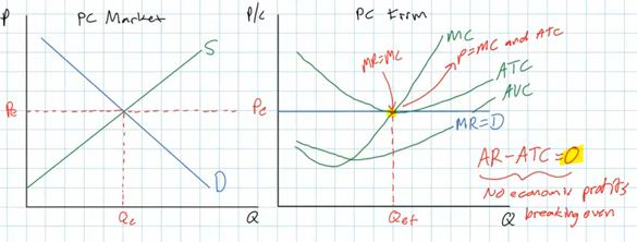
Long Run Equilibrium
A normal profit (zero economic profits) is what we would
expect individual firms in a perfectly competitive market to earn
in the long run because there are no barriers to entry.
And in long run equilibrium the P = MC (allocative efficiency,
more later) and P = minimum ATC (productive efficiency, more
later).
The individual firms are producing the quantity where their
costs per unit (the ATC) are the lowest.
if the firms produce any other quantity (less or more)
then the costs per unit (ATC) will be higher than the price and
they would earn economic losses [ME: meaning that they
could make more by quitting this business and going to their
next best alternative.]
Why do perfectly competitive firms only earn a normal profit in
the long run?
- What if they are earning short run profits due to an
increase in demand for their product?
- on the market graph the market demand will shift to the
right resulting in higher equilibrium market price
- on the graph for the individual firm the higher market
price is shown as a shift upwards of their perfectly elastic D=
P curve which is also their MR curve (D=P=MR)
- each individual firm then will respond to the higher market
price by producing a higher quantity since they will always try
to maximize their profits by producing where MR = MC, and this
now occurs at a higher level of output
- this higher price and quantity for each individual firm
will result in short run economic profits
- ME: with the higher price and quantity its total revenue
(TR) will be a lot higher
- its total costs (TC) will be only a little higher. Note
the ATC curve does not shift, but rather as firms increase
output they move slightly up their existing ATC curves
- and the yellow rectangle represents the firms new short
run profits caused by an increase in market demand
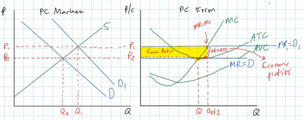
- But, what will happen in the long run?
- these short run economic profits will attract new
firms to the industry. REMEMBER: in pure competition
there are no barriers to entry so new firms can
easily enter the industry to try to capture some of these
economic profits.
- so, what will happen to our graphs if new
firms enter?
- one of the non-price determinants of supply is the
number of producers. If the number of producers goes up,
then the market supply will increase and shift to the
left.
- this will cause the market price to fall and the
P=D=MR curve for the individual firms to fall
- the individual firms then will no longer be earning
short run profits and in the long run they will be back
to zero, or normal, profits
- Entry Eliminates Profits
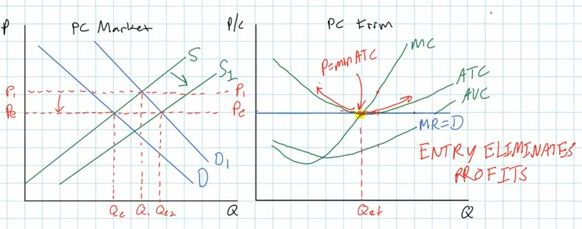
- ME: so what has happened in this perfectly competitive
industry in response to an increase in demand?
- Earlier we said: "The equilibrium quantity in the
market will be equal to the profit maximizing quantity
for the individual firms times the number of firms"
- because of the increase in demand and the increase in
supply that resulted from it the equilibrium quantity in
the market has increased from Qe to Qe2 on the graph
above.
- each individual firm is still producing the same
quantity as before (Qf) after temporarily producing a
larger quantity
- But, there are now more firms in the industry each
producing QF at the original price of Pe.
- This is good for consumers (society) . We wanted more
(increase in demand) and we got more at the same
price.
- What if they are earning short run losses due to a decrease
in demand for their product?
- Assume that initially all individual firms are earning zero
(normal) profits
- if demand decreases the market demand curve will shift to
the left and the equilibrium price will fall
- for the individual firms this means that their D-P- MR
curve will shift downward
- firms always want to maximize their profits so they will
produce the quantity where MR=MC, which is now at a lower
quantity
- and at this new profit maximizing quantity the price is now
below their ATC and they will now be earning economic losses.
- price is lower, so TR is lower
- ATC is now higher
- so their ATC is now > P
- ME: Price (P) and Average Revenue (AR) mean the same
thing
- and Profits = TR - TC = will be negative (economic
losses)
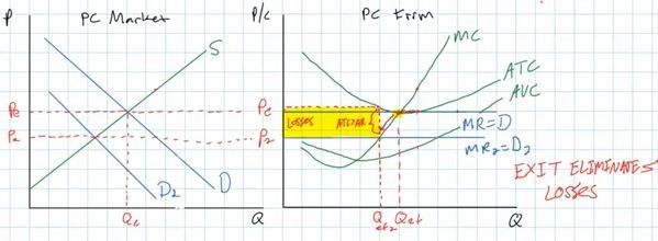
- How will firms respond to these short run economic losses?
- Exit Eliminates Losses
- due to the short run losses some firms will leave the
industry
- remember an economic loss means that they can make
more at their next best alternative
- and since there are no barriers to entry or EXIT, it
is easy for firms to leave and go to their next best
alternative
- this will decrease the number of producers and decrease
the market supply
- causing the equilibrium market price to increase
- for each individual firms this will shift their D = P =
MR curve upward
- and they will respond by producing where MR = MC which
will be at a higher quantity and they will be earning normal
(zero) profits again
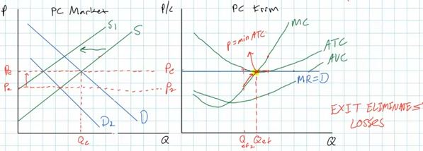
- after all adjustments the price will again be equal to
the minimum ATC, where the MC crosses the ATC
- and P = ATC = MC
- ME: So, in the long run in a perfectly competitive market
we will always get:
- normal (zero) profit
- P = minimum ATC
- P = MC
- Next lesson: Perfect Competition and Efficiency
Allocative and Productive
Efficiency in Perfectly Competitive Markets (econclassroom.com
19:35) - 8/9b
http://www.econclassroom.com/?p=3066
Why a firm in a perfectly competitive market will achieve
allocative and productive efficiency in the long run.
Introduction
- "In order to understand what makes less competitive markets
inefficient, we first must understand what it is that makes
perfectly competitive markets efficient."
- Imperfectly competitive markets: monopoly, oligopoly,
monopolistic competition
Review
- Productive efficiency:
- productive efficiency is producing at the lowest cost
- on a graph this is the lowest point on the ATC curve
(minimum ATC)
- this means the firm is using its resources wisely and not
wasting any resources
- "Productive efficiency occurs if the price of the good is
equal to the minimum ATC"
- ME: and, as we should already know, the MC curve crosses
the ATC curve at the lowest point of the ATC, so we find the
productively efficient quantity by finding the quantity where
MC = ATC
- Allocative Efficiency
- when the quantity of output produced achieves the greatest
level of total welfare (ME: satisfaction) possible
- producing the quantity where the consumer and producer
surplus is maximized
- ME: producing the quantity where MSB = MSC (marginal social
benefit = marginal social cost from chapters 3 and 5)
- ME : producing the quantity that maximizes society's
satisfaction
- ME: producing more of what people want and less of what
they don't want (more music downloads and less CDs)
How Perfectly Competitive Markets achieve Productive Efficiency in
the long Run
- Productive efficiency:
- productive efficiency is producing at the lowest cost
- on a graph this is the lowest point on the ATC curve
(minimum ATC)
- this means the firm is using its resources wisely and not
wasting any resources
- "Productive efficiency occurs if the price of the good is
equal to the minimum ATC"
- ME: and, as we should already know, the MC curve crosses
the ATC curve at the lowest point of the ATC, so we find the
productively efficient quantity by finding the quantity where
MC = ATC
- firms achieve productive efficiency if P = MC = ATC
- On the graph of a perfectly competitive firm in long run
equilibrium
- the firm will produce the4 quantity where MR = MC because
this is its profit maximizing quantity (Qf on the graph
below)
- and, we can see that the profit maximizing quantity is also
the quantity where the ATC is at a minimum (Qf on the graph
below)
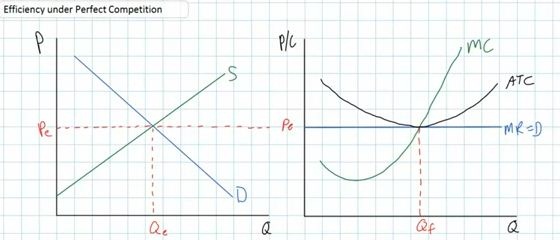
- So, purely competitive firms will achieve productive
efficiency in the long run
- what would happen if the price was higher than ATC?
- the firm would produce more
- and the profit maximizing quantity will not be at the
lowest point of the ATC curve; not where MC = ATC
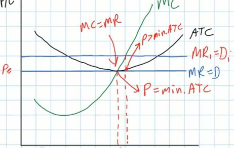
- so, in the short run this firm is not productively
efficient, but it is now earning economic profits
- and as we learned in the previous video lecture, these
profits will attract new firms, and because there are no
barriers to entry, this will increase supply and decrease
the price until each firm is again producing the quantity
where the P = minimum ATC
- and in the long run productive efficiency is achieved in
perfectly competitive markets (P = minATC)
How Perfectly Competitive Markets achieve Allocative Efficiency in
the long Run
- Allocative Efficiency
- definition of allocative efficiency:
- when the quantity of output produced achieves the
greatest level of total welfare (ME: satisfaction)
possible
- producing the quantity where the consumer and producer
surplus is maximized
- ME: producing the quantity where MSB = MSC (marginal
social benefit = marginal social cost from chapters 3 and
5)
- ME : producing the quantity that maximizes society's
satisfaction
- ME: producing more of what people want and less of what
they don't want (more music downloads and less CDs)
- consumer surplus (CS)
- is the total well being of consumers who are willing and
able to pay a higher price than the equilibrium price in the
market
- graphically consumer surplus is the area of the triangle
below the demand curve and above the equilibrium price (the
yellow area on the graph below)
- producer surplus (PS)
- is the total welfare of producers who are able to sell
their product at a price greater than their cots of
production
- is the total welfare gained by producers who were able to
sell their product a price higher than the price they were
willing to accept
- graphically, producer surplus is the area above the supply
curve but below the equilibrium price (the blue triangle on the
graph below)
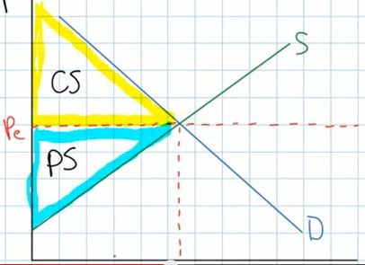
- So, in long run equilibrium a perfectly competitive market
will produce the quantity where consumer and producer surplus is
maximized and MSB = MSC
- if less is produced (Q1)
- we can see that MSB > MSC and this means too little is
being produced
- ME: I have use the terms MSB (marginal social benefit) and
MSC (marginal social cost) , here the instructor is calling
these just MB and MC
- if more than the long run equilibrium quantity is produced
(Q2):
- MSB<MSC (video MC>MB) and society would be better off
with less because the extra benefits that they are getting from
one more unit of output is less than its costs
- ME: remember that all costs are opportunity costs so if
MSB<MSC this means that the costs to society of producing
more are the lost benefits that we could have gotten if we
produced something else. If MSC are high this means that
something else would give us more satisfaction.
- and allocative efficiency is not achieved
- So allocative efficiency is achieved at that quantity where
MSB = MSC (MB = MC)
- this is also called the "socially optimal quantity"
- For the individual firm (the graph on the right)
- MSC = MC
- MSB = P
- so allocative efficiency is achieved where P=MC
- ME: why is the price we have to pay for a product a
benefit? Isn't that a cost?
- price is a benefit to the consumer because it measure
the benefits that the consumer is getting from the
product
- if consumers who are part of society get a lot of
benefits from a product they would be willing to pay more.
If consumers get few benefits from a product they would only
buy it if the price was less
- for example I would pay more to ski in the mountains of
Colorado (where I am now as I type these notes) than I would
pay to ski the hill of Wisconsin because I get more benefits
(more fun) skiing in Colorado
- ME:We know that all firms what to maximize profits so they
will produce the quantity where MR=MC. We can see on the graph
below that this perfectly competitive firm in long run
equilibrium will produce the quantity Qf to maximize its
profits. But note that this is also where P=MC.. So even though
all the firm was trying to do was to make as much money as
possible it will firm also achieve allocative efficiency. This
is the INVISIBLE HAND of competition that we talked about in
chapter 2.
- SUMMARY: Competitive firms achieve allocative efficiency in
the long run
- All firms will produce the quantity where MR=MC to maximize
their profits
- Because of the lack of barriers to entry, competitive firms
will receive only normal profits in t he long run
- But the long run profit maximizing quantity will also be
the allocatively efficient quantity:
- the quantity where P = MC,
- the quantity where MSB = MSC
- and the quantity where the sum of the consumer and
producer surplus is maximized
- WHY?
- perfectly competitive firms achieve allocative efficiency
in the long run because the demand curve for the individual
firm is perfectly price elastic
- i.e. they are "price takers"
- Since there are very many firms producing standardized
(identical) products, firms do not have any control over the
price of the product
- this means that each individual firm can sell all they
have at the market price
- This means that the P = MR
- since they don't have to lower their price to sell
more
- the extra revenue that they get when they sell one more
is the same as the price
- THEREFORE: when competitive firms try to find the
quantity where MR=MC to maximize their profits, it will also
be the quantity where P=MC. So when they maximize their
profits they also achieve allocative efficiency
- P = MR for perfectly competitive firms ONLY
- we will see in other product market models that the P
> MR, i.e. the price they receive is greater than the
extra revenue (MR) they get when they sell one more
- only for price takers with perfectly elastic demand
curves does the P always equal MR
- firms in other product market models must lower their
price to sell more so, as we will see in future chapters
P>MR
- therefore, when firms in the other market models produce
the quantity to maximize their profits (quantity where
MR=MC, it will not be the allocatively efficient quantity
(where P = MC).
- To understand this better, let's see what happens if the
competitive firms produce less than the profit maximizing quantity
(Q1 on the graph below).
- at Q1 we can see that MR does not equal MC so the
firm is not maximizing its profits
- in fact, we can see that ATC is greater than P , So TC will
be greater than TR and the firm is l
- earning a loss
- ALSO, P > MC so there is an underallocation of resources
toward this product. Too little is being produced. Remember, P
measures the MSB and MC measures the marginal social costs
(assuming that there are no externalities, so if P>MC then
MSB>MSC and society would be happier with more.
- Now if we assume that all firms are producing at Q1 on
their individual cost curves then the market quantity being
produced will also be less then the equilibrium. so on the
market supply and demand graph Q1 would be produced, not the
profit maximizing equilibrium quantity Qe.
- At this smaller quantity the MB to consumers is greater
than the MC
- This is allocative inefficiency because society is getting
less satisfaction
- Using the consumer and producer surplus model:
- allocative efficiency is achieved when the consumer and
producer surplus is maximized
- this occurs at the equilibrium level of output
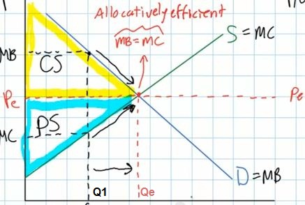
- but if the quantity is less than Qe, like Q1 then the
total consumer plus producer surplus is less (see the green
area on the graph below
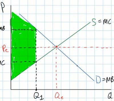
- and there is a loss of satisfaction to society (less
consumer and producer surplus) equal to the yellow triangle
on the graph below. this is what economists call the
"deadweight loss" of allocative inefficiency
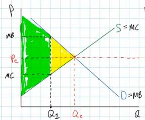
- We Since less than the efficient quantity is being
produced we say that resources are underallocated to
this product, i.e. society would gain satisfaction (equal to
the yellow triangle) if more resources were used so that
more was produced. This is allocative inefficiency.
- if firms produced more than the allocatively efficient
(and profit maximizing) quantity then again we would have
allocative inefficiency. This time MC will be > P, and
resources will be overallocated to the production of this
product. Too much is being produced. Society would be
happier if less of this was produced and more of something
else that gives us more satisfaction.
- in the market at Q2 on the graph below,
MSB<MSC
- ME: remember the opportunity cost (MSC) of consuming
this product is the satisfaction that you are not getting
from your next best alternative. So if extra benefits
that you are getting from this product (MSB or D) is less
than the benefits that you could get from something else
(MSC or S) then society would be better off with less of
this product. We say that resources are overallocated to
the production of this product.
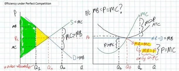
Perfectly competitive firms achieve both productive and
allocative efficiency in long run equilibrium
- they will produce the profit maximizing quantity where
MR=MC
- and this quantity will also be the productively efficient
quantity where ATC is at its minimum point
- and, this quantity will also be allocatively efficient where
P=MC
Chapters 10 and 18 - Pure Monopoly and Regulation
(Modules 10/18a and 10/18b)
10/18a - MONOPOLY: CHARACTIERISTICS AND SHORT RUN
EQUILIBRIUM
- MONOPOLY
- 9.1-1 Barriers to Entry - Defining Market Power [TW
6.1.1 (10:10)]
- 9.2-1 Defining Marginal Revenue for a Firm with Market
Power [TW 6.1.2 (12:43)]
- PROFIT MAXIMIZATION FOR A MONOPOLY
- 9.3-1 Determining the Monopolist's Profit Maximizing Output
and Price [TW 6.1.3 (14:18)]
- 9.3-2 Calculating a Monopolist's Profit and Loss [TW
6.1.4 (6:24)]
- OPTIONAL
MONOPOLY
9.1-1 [TW 6.1.1
(10:10)] Barriers to Entry - Defining Market Power -
10/18a
- Outline
- Market power
- Sole ownership
- Government created Monopolies
- Natural Monopoly
- Summary
- If a firm that has a highly desirable product and is the ONLY
producer, what price will the firm charge?
- a firm has market power if it is able to influence the
market price of its product
- the firm is able to set the price of its own product
- the firm is a price setter
- a monopoly is a single seller of a good or service
- monopolies are quite rare
- monopolies arise from one of three factors: ME: our textbook
calls these "barriers to entry")
- a firm that has sole ownership of a particular resource
used to produce a good
- e.g. diamonds: the deBeers diamond company owned almost
80% of the world's diamond mines
- e.g. if one company owns the only place for selling
concessions in an airport
- a monopoly that is created by government action like
patents, copyrights, or special licenses
- e.g. pharmaceuticals companies that develop a new drug
receive a patent to be the sole seller for a certain length
of time
- sole licenses granted by the government to one company;
e.g. the Hudson Bay Company
- a natural monopoly arises because of the interaction
between the size of the market and the efficient scale of
operation of a single firm
- the lowest point of the long run average cost curve show
the efficient scale, or "right size" for a firm in the long
run
- ME: this is the productively efficient quantity where
costs per unit are minimized. Recall that productive
efficiency means producing at a minimum cost. The
productively efficient quantity then occurs in the long run
where the MC crosses the ATC (MC=ATC)
- note that this is what happens in the long run for
purely competitive firms
- if the point of efficient scale (productively efficient
quantity) is small compared to the total demand in the
market then there can be many firms int he industry
providing this product, ALL producing at the point of
efficient scale (Productive efficiency)
- BUT, in a natural monopoly just ONE FIRM can produce
everything that is demanded and point of efficient scale
(the minimum point on the long run average cost curve ) is
BEYOND the demand curve. See how the demand curve crosses
the LRAC curve where it is still going down
- this occurs when the industry has very large economies
of scale (the LRAC curve is downward sloping over a wide
range of output. This is a natural monopoly because it makes
for ether to be just one firm producing the product because
one firm (a monopoly) can produce all that society demands
at a lower cost than if ether were more firms in the
industry
- examples include: electrical utilities (in the past) two
sets of wires running to each house i f there were two
companies would be more costly
9.2-1 [TW 6.1.2
(12:43)] Defining Marginal Revenue for a Firm with Market Power -
10/18a
- Outline
- Marginal revenue defined
- Total revenue
- Marginal revenue table
- Graphing marginal revenue
- Summary
- Example: you have a monopoly - the only restaurant in an
airport
- Problem: what price do you charge to maximize profits?
- if you charge too high of a price many people might just
fly hungry
- if you charge too low of a price you will attract more
customers, but you will make less on each one
- marginal revenue is the change in total revenue that results
form selling one more unit of output
- MR = change in TR / change in Q
- the P and Q columns are your demand curve
- calculate TR = P x Q
- ME why does the TR begin to decrease at very low prices?:
because demand is inelastic
- calculate MR = change in TR / change in Q
- ME: MR is the slope of the TR graph
- MR is negative when TR falls as you lower the price too low
and TR decline (demand in price inelastic)
- How can you have less revenue when you are selling
more
- Graph:
- the demand curve
- downward sloping like in chapter 3
- D=P=AR
- average revenue: AR = TR/Q
- AR is the same as price
- the MR curve
- ME: our textbook plots the MR points at the midpoints
!!
- the MR is less than the price, ALWAYS
- the MR curve lies below the demand curve
- Why?
- why is the MR (the extra revenue that we get when we
sell one more unit) less than the price at which we sold
it?
- because in order to sell more the firm has to lower
the price on ALL units
PROFIT MAXIMIZATION FOR A
MONOPOLY
9.3-1 [TW 6.1.3
(14:18)] Determining the Monopolist's Profit Maximizing Output
and Price - 10/18a
- Outline
- Marginal revenue curve
- Graphing total revenue
- Marginal cost curve
- Point of maximum profit
- Problem for a firm with market power: what price do you charge
to maximize profits?
- if you charge too high of a price many people might just
fly hungry
- if you charge too low of a price you will attract more
customers, but you will make less on each one
- How does a profit maximizing monopolist choose the price for
which it sells its product and the quantity that it sells?
- ME: we will be using benefit-cost analysis. It will continue
to produce (and increase its profits) as long as the extra
benefits that it receives (MR) is greater than the extra costs
(MC)
- Review of MR: see above
- marginal revenue measures the extra benefits that a
monopolist gets when it sells one more unit of its product
- remember: marginal revenue is always less than the
price
- What if there is no cost to produce the product?
- in pure competition the price of a free product would be
free; this would be where P{=MC because MC would be zero
- but a monopolist selling a product that has no cost to
produce, then you have market power and then "you can maximize
profits by charging a price equal to what the market will
bear"
- how to calculate TR and show on a graph
- as long as your extra benefits, which in this case is the
MR is greater than zero (the extra cost), the monopolist is
adding revenue to its profits and profits will increase. when
MR = 0, then the TR are maximized.
- So if costs = 0, a profit maximizing monopolist will
produce where its MR = 0; then the produce the quantity where
MR = 0
- But what if there are costs? To maximize profits you may
not want to maximize your TR because your profits depend on TR
and TC
- add the marginal cost curve to the graph
- and produce as long as the MR is greater than the MC; the
profit maximizing quantity is the quantity where MR = MC
!!!!! Know this !!!!!!
- keep producing more if MR > MC
- never produce where MR < MC because this will make your
profits smaller
- the profit max Q is where MR=MC
- yes, this last unit (marginal unit) is adding nothing to
your profits
- but, if you produce where MR=MC you know that you have
also produced ALL the units where MR > MC and this will
maximize the profits
- how do you find the price that the monopolist will charge
for the profit maximizing quantity? To find the price you must
go up to the demand curve at the Qprofmax
- ME: in pure competition you did not have to go up to the
demand curve to find th price because the demand curve was
horizontal, BUT for all other market models you MUST get the
price from the D or P curve.
9.3-2 [TW 6.1.4
(6:24)] Calculating a Monopolist's Profit and Loss -
10/18a
- Outline
- Average total cost curve
- Calculating profit
- Graphing profit
- Monopoly with a loss
- to maximize profits a monopolist will produce the quantity,
and charge the price, where MR=MC
- charging the "profit maximizing price" does not guarantee a
profit; monopolies can earn losses, but the MR=MC rule will
minimize losses
- good review of the ATC curve
- a monopolist earning a profit
- profit = TR - TC
- TR = P x Q
- ME: I do not stress the "per unit profit" or "profit
margin"; it just seems to be an additional step that is not
necessary
- be able to find the following on the graph: Q, P, ATC,
TC, TR and profit
- especially the TR, TC, and profit rectangles
- REMEMBER: once you find the quantity where MR=MC you must
got up to the demand curve to get the price
- a monopolist earning a loss
- be able to find the following on the graph: Q, P, ATC,
TC, TR and loss
- especially the TR, TC, and loss rectangles
- ME: the video lecture does not discuss the shut down
situation. See the textbook for this.
- Summary
- a monopoly will maximize profits by producing where
MR=MC
- if the P > ATC then the monopoly will make a profit
- if the P < ATC then the monopoly will make a loss
MODULE
10/18b - MONOPOLY: LONG RUN EQUILIBRIUM, EFFICIENCY, AND
REGULATION
- THE SOCIAL COST OF MONOPOLY
- REGULATING NATURAL MONOPOLIES
THE SOCIAL COST OF
MONOPOLY
9.4-1 [TW 6.2.1
(12:22)] Determining the Social Cost of Monopoly - 10/18b
- Outline
- The missing supply curve
- Price in a competitive market
- Price in a monopoly
- Costs imposed by the monopoly
- Introduction
- why are monopolies so unpopular?
- maybe because they are imposing costs on society
- ME: the textbook discusses how monopolies, in the long run,
are allocatively and productively INEFFICIENT, that is:
- they do not produce the quantity that would maximize
society's satisfaction = dead weight loss (allocative
efficiency); monopolies will charge a higher price and
produce a smaller quantity than if we had a competitive
market
- the do not produce at the minimum cost (productive
efficiency
- The missing supply curve
- what does "supply" mean in economics (see chapter 3)
- monopolies are price setters therefore there is no supply
curve
- monopolies are not given a price, they set the price
- Price in a competitive market
- ME: If this market were competitive (chapters 8 and 9),
then if the price were high and profits existed, new firms
would enter (remember: no barriers to entry) and this would
drive the price down to the MC. What quantity would a
competitive firm produce? The quantity where P=MC (or demand =
MC). This is the allocatively efficient quantity. According to
the textbook allocative efficiency occurs when P=MC. Purely
competitive firms are allocatively efficient. Are
monopolies?
- be able to find the price and quantity that would occur if
the market were competitive because this is where "economic
value" is maximized. ME: our textbook uses the term "allocative
efficiency".
- The demand curve measures the benefits that that consumers
get from a unit of the product and the MC curves measures the
costs of producing that extra unit. As long as the marginal
social benefits (MSB) are greater than the marginal social
costs (MSC), society is gaining satisfaction. Society's
satisfaction is maximized where MSB=MSC, or on our graph, where
P=MC (assuming no externalities exist) ME: this is what our
textbook calls the allocatively efficient quantity. But do we
get this quantity if this were a monopoly?
- Price in a monopoly
- a monopoly will produce the quantity that maximizes its
profits; the quantity where MR=MC
- the monopoly's profit maximizing quantity is LESS THAN the
quantity that maximizes society's satisfaction (where MSB=MSC
or where P=MC)
- you should be able to find the profit maximizing quantity
(WHAT WE GET) on the graph and the allocatively efficient
quantity (WHAT WE WANT)
- this imposes a cost on society because less will be
produced. A monopoly will not produce additional units EVEN
THOUGH the MSB of those units is greater than the MSC (or the
demand is above the MC)
- monopolies try to maximize profits, not maximize society's
satisfaction (allocative efficiency) they therefore produce
less and charge a higher price
- Costs imposed by a monopoly
- the loss triangle
- the area under the demand curve and above the MC curve of
the quantities that the monopolist does not produce even though
the benefits are greater than the costs -- so society
loses
- called a dead weight loss
- Monopolies will:
- produce less
- impose a dead weight loss on society
- monopolies are bad for society because they will produce
less than if the market were competitive and the loss of
satisfaction to society as a result is the dead weight
loss
- ME: monopolies do not produce the allocatively efficient
quantity
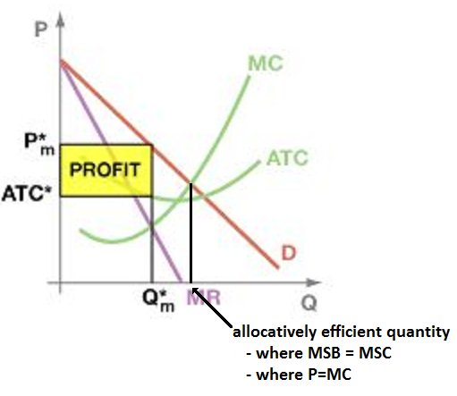
- on the graph above you can see that the profit
maximizing quantity (Q*m) is less than the
allocatively efficient quantity
- ME: the video lecture did not discuss how monopolies are also
productively inefficient, which means that they do not produce the
quantity that will minimize ATC (the don't produce the quantity
where MC=ATC). This is discussed in the textbook.
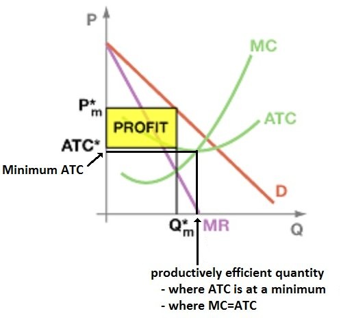
- on the graph above you can see the the ATC at the
profit maximizing quantity (ATC*) is higher than the
minimum ATC
9.4-2 [TW 6.2.2
(15:23)] Calculating Deadweight Loss - 10/18b
- Outline
- Economic value in a competitive market
- Economic value in a monopoly
- Calculating the deadweight loss
- Rent seeking
- Tomlinson assumes:
- constant marginal costs just to keep things simple
- no externalities, therefore the MC measures all of the
marginal social costs (MSC); stated a different way: private
costs = social costs
- the demand curve shows the reservation prices of consumers,
that is, the highest prices that consumers are willing to pay;
which means the demand curve measures the maximum benefits the
consumers get from the product, or the marginal social benefits
(D=MSB) assuming no externalities
- Economic value (efficiency) in a competitive market
- what price and quantity will occur in a competitive
market?
- The video lecture will ask you a
multiple choice question. ANSWER THE QUESTION by selecting A,
B, or C and more of the lecture will follow
- P=MC in a competitive market
- this is where the supply and demand cross (remember the
MC curve is the supply (horizontal in this example)
- ME: the is also the allocatively efficient quantity
because P=MSB and MC = MSC, do MSB = MSC
- no profit
- but a lot of consumer surplus; consumers do not have to
pay the maximum that they are willing to so they are gaining
satisfaction; Tomlinson calculates the consumer surplus
- economic value equals the consumer surplus plus the
producer surplus (here there is no producer surplus)
- Economic value in a monopoly
- what price and quantity will occur in a monopolistic
market?
- monopolies will try to maximize their profits
- this will maximize the producer surplus, BUT reduce the
total economic value for society
- assumes that this is a "one-price" monopolist: i.e.
there is no price discrimination (see textbook)
- when maximizing profits the monopolist will produce less
than if the market were competitive
- this then will reduce the economic value for society
since there will be less consumer surplus because less is
produced
- this loss of economic value (consumer surplus in this
example) is called dead weight loss
- Monopolies will maximize their profits by raising the
price and reducing output ("restrict trade) which will drive
some customers out of the market and society loses their
consumer surplus
- ME: this represent allocative inefficiency since at the
profit maximizing quantity for the monopolist, the P (or
MSB) is greater then the MC or MSC (P>MC or MSB>MSC;
society wants more of the product and the cost to society is
low indicating that ether are additional units when the
benefits outweigh the costs that society is not getting
- Rent Seeking
- this is another social cost of monopolies (ME: another
source of inefficiency)
- "rent seeking" refers to actions that firms take to
preserve their profits (ME: called "monopoly preserving
expenditures" in our textbook
- additional resources are used, NOT to benefit society, but
just to preserve the monopoly, this is a loss to society
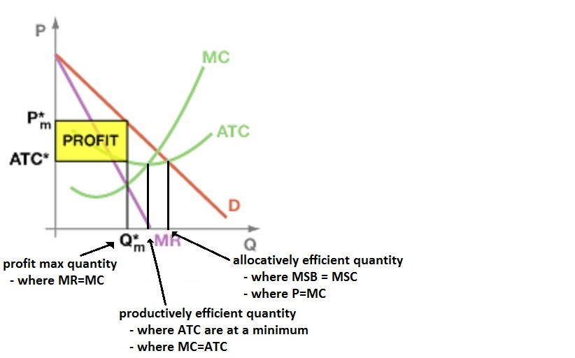
Price Discrimination and
its Effects on Efficiency in a Monopolistic Market
(econclassroom.com 14:51) - 10/18b
http://www.econclassroom.com/?p=3118
Outline:
- Define price discrimination
- Three conditions necessary for price discrimination
- Three types (degrees) of price discrimination
- The effect of perfect price discrimination on efficiency
(graph)
Definition: Price discrimination occurs when a firm with market
power charges different prices to consumers for an identical
product.
ME: Note that the word "discrimination" does not mean
that this is a bad thing. All "discrimination" means is that
different customers are treated differently, i.e. they pay
different prices. We will find out that price discrimination may
actually be GOOD for society.
Examples:
- Movie theaters: Charge different prices based on age.
Seniors and youth pay less since they tend to be more price
sensitive.
- Gas stations: Gas stations will charge different prices in
different neighborhoods based on relative demand and
location.
- Quantity discounts: Grocery stores give discounts for bulk
purchases by customers who are price sensitive (think “buy
one gallon of milk, get a second gallon free”& the
family of six is price sensitive and is likely to pay less per
gallon than the dual income couple with no kids who would never
buy two gallons of milk).
- Hotel room rates: Some hotels will charge less for
customers who bother to ask about special room rates than to
those who don’t even bother to ask.
- Telephone plans: Some customers who ask their provider for
special rates will find it incredibly easy to get better
calling rates than if they don’t bother to ask.
- Airline ticket prices: Weekend stayover discounts for
leisure travelers mean business people, whose demand for
flights is highly inelastic, but who will rarely stay over a
weekend, pay far more for a round-trip ticket that departs and
returns during the week.
Three conditions necessary for price discrimination to occur:
- firm must have market power (therefore purely competitive
firms cannot price discriminate, but monopolies can
- firm must be able to segregate customers with different
willingnesses to pay which means with different price elasticities
of demand
- ME:
- those with a less elastic demand are charged a higher
price. So what happens to total revenue (TR)? We know that
if demand is inelastic and price goes up, TR increase.
- those with elastic demand are charged a lower price. So
what happens to TR? We know that if demand is elastic and
price goes down, TR increase.
- Our textbook defines price discrimination as "the
selling of a product to different buyers at different prices
when the price differences are not justified by
differences in cost.
- so charging more for a car in Alaska and less for one
in Detroit because it costs more to ship the car to
Alaska is NOT price discrimination
- But, since we assume that the costs (TC) are the same,
the result of price discrimination is higher TR with the
same TC, So, HIGHER PROFITS
- buyers are prevented from reselling the product to someone
else
Example: Airline tickets
ME: airlines have market power which means that they can
set their own price
ME: business travelers have a less elastic demand curve than
vacation travelers, but how can the airline know if a ticket buyer
is a business traveler or a vacation traveler? One way is to
require a Saturday night stay for customers buying round-trip
tickets. Business travelers prefer to be home on weekends and
vacation travelers tend to want to be on vacation over the
weekend
resale is prevented because your name is on the ticket and you
must have a matching ID
Three types (degrees) of price discrimination
3rd Degree: where consumers are divided into GROUPS. For
example, age groups with different price elasticities
(movies tickets are cheaper for children and more expensive for
adults), or time of purchase (people who buy early pay less
than those who buy at the last moment).
2nd Degree: where price discrimination is based on the quantity
purchased. For example, buying in bulk (large quantities)
is cheaper than buying small quantities or two-for one (or
buy two get one free). the more you buy the less you pay per
unit
1st Degree: Also called "Perfect Price Discrimination". This is
where each individual consumer pays a different price, each
consumer pays the highest price that he or she is willing to pay
based on their demand. This way there will be no consumer surplus
but a lot of producer surplus.
The Effect of Perfect Price Discrimination on Efficiency (graph
showing 3rd degree price discrimination)
REVIEW: Graph of a "single-price" monopolist maximizing
profit. "Single-price" means that there is no price discrimination
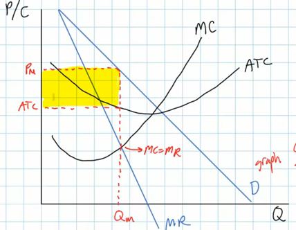
So, if this monopolist did not price discriminate they would
produce quantity Qm and charge price Pm. (They will produce the
quantity where MR=MC.) ME: and at Qm, P > MC so the
monopolist is not allocatively efficient.
PRICE DISCRIMINATION: But notice that the demand curve goes
above Pm, meaning that there are customers willing to pay more
than Pm. What would happen if the monopolist could charge these
customers more since they are willing to pay more? What happens
is: if the monopolist can charge each customer the highest
price that they are willing to pay, then MR will be the same as
price (or demand). D = MR or P = MR
So, what quantity will the perfectly price discriminating
monopolist produce to maximize profits? This is always where
MC=MR. Always.
On the graph, if P = MR then MR = MC where P = MC. You
should remember that this is the formula used to find
allocative efficiency (the socially optimal quantity)
Results of perfect price discrimination:
- more will be produced than a single-price monopolist
(Qp=MC on the graph below)
- some consumers will pay higher prices than they would if
there was no price discrimination (Pm), but other consumers
will pay lower prices
- profits will be greater (the blue plus the yellow areas
on the graph below)
- AND MOST IMPORTANTLY the perfectly price discriminating
monopolist will produce the allocatively efficient quantity!
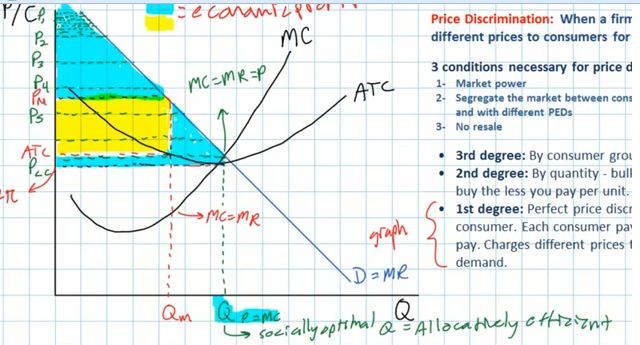
Conclusion:
- 1st degree price discrimination is almost impossible and
therefore very uncommon.
- 2nd and 3rd degree price discrimination are more
common
- but, 2nd and 3rd degree price discrimination do not
achieve the same increase in output as perfect price
discrimination and therefore do not achieve the same level
of allocative efficiency, but they are still better than a
single-price monopolist.
- effects:
- more is produced
- consumer surplus is transferred to the producers in
the form of higher revenues and profits
- Is price discrimination good for society? it depends:
- YES - it is better for the monopolist because they
get higher profits
- YES - it does improve allocative efficiency
- NO - if you are one of the customers who has to
pay an even higher price
- YES - if you are one of the customers who gets the
product at a lower price, and if there were no price
discrimination, you would not get the product at
all
REGULATING NATURAL
MONOPOLIES
Natural Monopoly and the need for Government Regulation -
10/18b
http://www.econclassroom.com/?p=3115
What is a "Natural Monopoly"?
- Monopoly where the long run ATC curve has economies of scale
over a very large range of output
- You can identify the graph of a natural monopoly because
the demand (D) curve crosses the ATC curve when the ATC is still
downward sloping
- this means that one very large company can produce every thing
that is demanded AT AT LOWER AVERAGE COST than if there were
several competing firms
- Examples:
- providing water to homes in a city
- electrical utilities
- natural gas
- If there were many companies each serving only a few customers
the ATC (costs per unit of output) would be higher
- it would make more sense to have only one company provide the
product because then the costs per unit (ATC) would be lower. That
is why this is called a "natural" monopoly.
- this is because there are very high fixed costs (TFC). Think
of all the costs of running water pipes to every house in a city.
These are all fixed costs. And since the TFC are very very high,
then the TC will be very high, and the only way to get ATC to be
low is to have a large amount of output (Q)
- ATC = TC / Q
- if TC are very high because of very high TFC then:
- ATC is high if: ATC = high TC / low Q
- but, ATC would be low if : ATC = high TC / large Q
Compare graphs:
- graph of a regular monopoly
- graph of a natural monopoly (EoS - Economies of Scale)
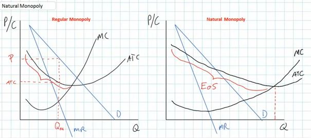
So, Society is better off (lower costs) if only one firm produces
the product, BUT:
- what will a profit maximizing monopolist do is such a
case?
- they would produce the profit maximizing quantity, where MR =
MC
- and this is NOT the allocatively efficient quantity
- like other monopolists, a natural monopolist will charge a
higher price (Pm) and produce a lower quantity (Qpm) than the
socially optimum (alloc. eff.) price of Pso and quantity of
Qso
- Result: allocative inefficiency; an underallocation of
resources
- ME: so WHAT WE GET (Qpm) is less than WHAT WE WANT (Qso)
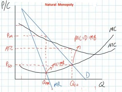
To really benefit society, natural monopolies need to be regulated
by the government
- This means that the government should use price controls and
subsidies to achieve allocative efficiency, Qso
- But what price should the government select?
- if the government puts on a price ceiling at the
allocatively efficient price of Pso
- the monopolist would then produce the allocatively
efficient quantity of Qso because the ceiling price becomes the
firm's MR and then MR = MC at Qso
- BUT, we can see that at Qso the ceiling price is less than
the ATC and the monopoly would be earning losses equal to the
blue rectangle on the graph below
- in the long run, businesses cannot operate at a loss and
they will go out of business. This would not be good for
society.
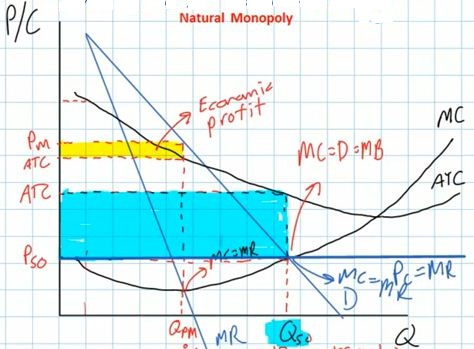
- What can the government do to prevent natural monopolies from
going out of business because to the price ceiling?
- they can use BOTH a price ceiling AND a subsidy to help the
monopoly produce the socially optimum quantity.
- ME: our textbook does NOT use the subsidy graph shown in
the video lecture (see below)
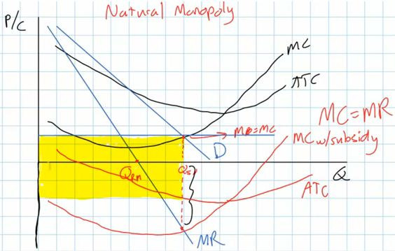
- ME: our textbook says that there are two solutions to the
problem of natural monopolies earning a loss at the
allocatively efficient price:
- provide a subsidy to cover their losses
- but this may be politically unpopular. Would you
support higher taxes to give money to Commonwealth Edison
electric company?
- the other solution that is used a lot in the united
states is AC pricing, where the government does not set a
price ceiling at the allocatively efficient price (Pso), but
rather they put the price ceiling at a prise where D=ATC
(where the demand curve crosses the ATC curve).
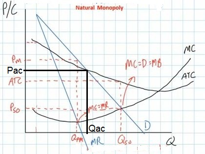
- If the price is Pac then the firm will produce Qac
- is the allocative efficient? NO, but it is closer to
Qso
- will the firms earn profits or losses? They will earn
normal profits (profits = zero) and they will be able to
stay in business. (Remember: economic costs include the
explicit costs AND the implicit cost which means that
investors are earning a return on their investment
approximately equal to their next best alternative.)
Chapter 11 - Monopolistic Competition and
Oligopoly (Modules 11a and 11b)
MODULE 11a - MONOPOLISTIC COMPETITION
- MONOPOLISTIC COMPETITION
- 10.1-2 Defining Monopolistic Competition [TW 6.4.1
(7:01)]
- 10.2-1 Short-Run Profit Maximization for a Monopolistically
Competitive Firm - Understanding Pricing and Output in
Monopolistic Competition [TW 6.4.2 (8:58)]
- Monopolistic
Competition (econclassroom.com 20:51)
efficiency begins at 15:00
- Monopolistic Competition in the Long-Run: Econ Concepts in
60 Seconds with AP Economics Teacher (ACDCEcon 3:25)
http://www.youtube.com/watch?v=erdzOu3juNI
10.1-2 [TW 6.4.1
(7:01)] Defining Monopolistic Competition - 11a
- Outline
- A Review of Two Market Types
- Definition of Monopolistic Competition
- Product Differentiation
- How to Create Market Power
- A Review of Two Market Types
- Monopoly: because of barriers to entry they have market
power [MR=MC] and can earn long run economic profits,
but they create less economic value for society (ME:
allocatively [P>MC] and productively [not
minimum ATC] inefficient in the long run)
- Perfect Competition: because there are no barriers to entry
they earn zero economic profits int the long run (ME: called a
normal profit), but they maximize economic value for society
(ME: they are allocatively [P=MC] and productively
[P=MC=ATC] efficient in the long run)
- Definition of Monopolistic Competition
- Simple Definition: a market in which firms can enter freely
and obtain market power by differentiating their product
- Some market power but no (or few) barriers to entry
- firms compete to create little monopolies
- firms have to convince their customers that their product
is distinct; this gives the firm a downward sloping demand
curve and some market power
- a hybrid of monopoly and competition
- from monopoly: MR=MC ; the result of market power
because of product differentiation
- from competition: P=ATC in the long run; i.e. firms earn
zero economic profits in the long run because there are no
barriers to entry
- explains how variety arises in a market
- Product Differentiation
- two different hamburgers look similar BUT: companies
advertise to convince customers that their hamburger is
different
- Pepsi vs. Coke, they are very similar BUT: companies
advertise to convince customers that their soft drink is
different
- How to Create Market Power
- why do firms spend so much money on product
differentiation, i.e. on trying to convince customers that
their product is distinct or different?
- because this creates market power; the ability to increase
a product's price without losing all of its customers; creates
little monopolies
- How:
- advertising
- actual differences in the product itself
- Result:
- a little more inefficiency than in perfect competition
which reduces society's satisfaction
- but more variety which increases society's
satisfaction
10.2-1[TW 6.4.2
(8:58)] Short-Run Profit Maximization for a Monopolistically
Competitive Firm - Understanding Pricing and Output in Monopolistic
Competition - 11a
- Outline
- The graph of a single firm
- Free entry into the market
- A shift in the demand curve
- Equilibrium in monopolistic competition
- The pros and cons of monopolistic competition
- The graph of a single firm
- downward sloping demand curve because of product
differentiation
- product differentiation gives the firm a kind of
monopoly
- because demand is downward sloping the marginal revenue
(MR) curve is below the price
- add the cost curves
- to find the Q and P, this profit maximizing firm will
produce the Q where MR=MC and the price is found on the demand
curve above. Know how to do this!
- know how to find profits or losses
- Free entry into the market (a long run change)
- there is only room in the market to support a certain
number of producers
- but since there are no barriers to entry if existing firms
are earning economic profits then new firms will enter the
industry AND WHAT WILL HAPPEN THEN?
- A shift in the demand curve
- the demand for the existing firms will decrease (shifts to
the lift) also decreasing the MR
- result: quantity, price, and profits for firms in the
industry will decrease
- as long as firms are earning economic profits more firms
can enter and again causing Q, P and profits to decrease.
- where is the new equilibrium? when will it stop? when will
new firms stop entering the industry?
- Equilibrium in monopolistic competition
- Answer: when firms are l]no longer earning profits;
when economic profits are zero (or normal profits PAUSE the
video and look at the new graph carefully
- P = ATC and profits = 0 (breaking even) like in pure
competition
- the demand curve is tangent to the ATC curve
- and no new firms will enter, this is an equilibrium
- The pros and cons of monopolistic competition in the long run
- Is the new long run equilibrium good or bad for
society?
- Pros: a lot of variety, product differentiation, which will
give society some satisfaction
- Cons:
- not producing at the point of minimum ATC (not achieving
productive efficiency); costs are higher wasting some
resources
- also we are not producing where P=MC (not allocatively
efficient); there is a dead weight loss; less is produced;
there are still some quantities where the MPB (or P) is
greater then the MSC (or MC) representing lost satisfaction
for society
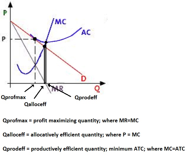
Monopolistic Competition
(econclassroom.com 20:51) - 11a
http://www.econclassroom.com/?p=3128
(efficiency begins at 15:00)
beginning at 15:00
- Are monopolistically competitive firms efficient?
- Graph of a monopolistically competitive firm in long run
equilibrium
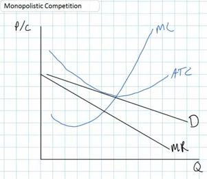
- firms earn a normal (zero) profit because of few
barriers to entry (P=ATC means zero profit)
- therefore there is no incentive for other firms to
enter
- Are they efficient? NO. Neither allocative or productive
efficiency will be achieved by monopolistically competitive
firms in the long run.
- Productive efficiency is NOT being achieved
- the profit maximizing quantity (Q) is not at the
lowest point on the ATC curve. The lowest point is where
MC-ATC (Qpe on the graph below)
- so to maximize profits, monopolistically competitive
firms will restrict output and charge a slightly higher
price than the minimum ATC
- Allocative efficiency is NOT being achieved
- We know that allocative efficiency occurs where MB=MC
(or MSB=MSC). On the graph MSB is measured by the demand
(or price) curve and the MSC is measured by the MC curve.
So, allocative efficiency occurs at the quantity where
P=MC.
- At the profit maximizing quantity we d]can see
that P>MC or MSB>MSC, so the firm is NOT
allocatively efficient.
- There will be an underallocation of resources (too
little will be produced). The quantity where P=MC (Qso)
is greater than the profit maximizing level of output
(Q).
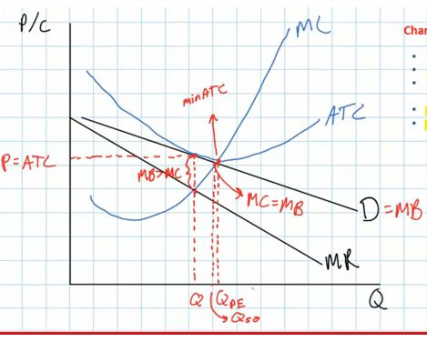
- We will always get productive and allocative
inefficiency when the demand curve is downward
sloping so the MR is less than the price (demand)
- Only in pure competition do we get productive and
allocative efficiency
Monopolistic Competition in
the Long-Run: Econ Concepts in 60 Seconds with AP Economics
Teacher (ACDCEcon 3:26) - 11a
http://www.youtube.com/watch?v=erdzOu3juNI
- How to draw a monopolistically competitive firm's long run
equilibrium graph
- downward sloping demand
- MR is below the Demand
- MC goes down at first ant then up
- IMPORTANT: NOW you must find the profit maximizing price and
quantity before you draw the ATC curve
- find the quantity where MR=MC
- then drive up to the demand curve and over to get the
price
- we need to know the price before we draw the ATC
curve
- then draw the ATC curve tangent to the demand curve (just
touching but not crossing) at the the profit maximizing price
(sweet spot).
- Now find the socially optimal quantity (the allocatively
efficient quantity)
- the alloc. eff. quantity occurs where P = MC. (On the video
he says this is "where supply equals demand" and he shows that
MC=S. This is the same as P=MC [or MC=P])
- result. the profit maximizing quantity, Q, (WHAT WE GET) is
less than the allocatively efficient quantity, Qso
(WHAT WE WANT).
- there is a deadweight loss
- Now find the productively efficient quantity
- this is at the minimum point of the ATC, or where
MC=ATC
- notice that the profit maximizing quantity is less than the
quantity where ATC is at a minimum, so monopolistically
competitive firms are not productively efficient. They do not
produce at the lowest ATC
- The difference between these two quantities is called
"excess capacity" meaning the firm could produce more at a
lower cost but they hold back production to increase their
profits
- Classic mistake when drawing the graph of monopolistic
competition in long run equilibrium:
- the classic mistake is drawing the ATC tangent to where
demand hits the MC curve
MODULE 11b -
OLIGOPOLY and SUMMARY OF PRODUCT MARKET MODELS
11.2-1 [TW 6.3.1
(17:26)] Introducing Oligopoly and the Prisoner's Dilemma -
11b
- Outline
- Oligopoly Defined
- Game Theory: The Prisoner's Dilemma
- Nash equilibrium
- Definition of Dominant Strategy
- Conclusion
- Oligopoly Defined
- SLIGHT ERROR: Tomlinson mentions that a monopolistically
competitive industry has "a small number of sellers" each with
some market power; he meant to say "a LARGE number of
sellers".
- Oligopoly
- small number of sellers
- that have to consider the reactions of their
competitors;
- they interact strategically
- ME: our textbook uses the term "mutual
interdependence";
- where each firm tries to guess what its competitor's
are going to do,
- because the choices of all the firms affects each
individual firm
- there is no generally agreed upon single model of
oligopoly: there are several models each with strengths and
weaknesses
- Game Theory: The Prisoner's Dilemma
- economists tend to agree that Game Theory best describes
strategic behavior between a small number of firms
- the Prisoner's Dilemma is one of the most basic forms of
game theory and it applies quite will to the strategic behavior
of a small number of firms (i.e. oligopoly) when they are
making their pricing decisions
- Bonnie and Clyde: confess or not confess?
- called a "game" because the outcome depends not just on
what you do, but what your competitor does; also called
strategic interaction
- draw a matrix (table) with two players representing the
possible outcomes in each box; prisoners cannot talk to each
other and they don't know what the other will choose
- each can either confess or not confess
- if both confess they will get 10 years in prison
each
- if neither confess then they will get only 1 year in
jail on a lesser charge
- if Bonnie confesses and Clyde doesn't, then Bonnie is
free (no jail time) and Clyde will get 11 years in
prison
- if Clyde confesses and Bonnie doesn't, then Clyde is
free (no jail time) and Bonnie will get 11 years in
prison
- Matrix of strategies available to each player:
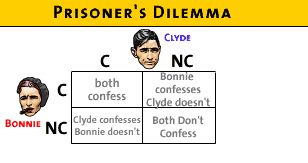
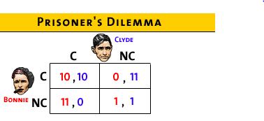
- Nash equilibrium
- What is the solution?
- Nash Equilibrium:
- the outcome when each player is doing the best they can
given what all other players are doing
- If Clyde confesses what is the best response for bonnie?
- The video lecture will ask you
a multiple choice question. ANSWER THE QUESTION by
selecting A, B, or C and more of the lecture will
follow
- If Clyde does not confess which is the best response for
Bonnie
- The video lecture will ask you
a multiple choice question. ANSWER THE QUESTION by
selecting A, B, or C and more of the lecture will
follow
- Definition of Dominant Strategy
- In both cases, Bonnie will minimize jail time by
confessing; this is Bonnie's "dominant strategy"
- Dominant Strategy: a choice for a player that
maximizes her satisfaction no matter what her rivals are
doing
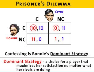
- What should Clyde do?
- The video lecture will ask you
a multiple choice question. ANSWER THE QUESTION by
selecting A, B, or C and more of the lecture will
follow
- Clyde will also have a dominant strategy of
confessing no matter what Bonnie does
- So they will BOTH confess = Nash equilibrium
- Nash equilibrium occurs when they both give their
dominant response
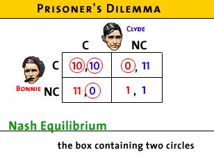
- it is also a "self-enforcing agreement": when they
are each giving their best decision, neither can improve
their situation by changing their minds
- so they will not change their minds; it is an
equilibrium
- BUT is this equilibrium the BEST for Bonnie and Clyde?
- The video lecture will ask you
a multiple choice question. ANSWER THE QUESTION by
selecting A, B, or C and more of the lecture will
follow
- It would be best if they would both NOT CONFESS,then
they each get only 1 year in prison rather than 10
years
- but it is not a Nash equilibrium because they can
each do better if they confess.
- they can do better because if one confesses and
the other does not then he or she will get no jail
time (0 years)
- so they will confess = Nash equilibrium
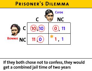
- The BEST outcome for both is not an equilibrium
outcome
- How does this apply to economics and business?
- businesses try to form trusting relationships so in a
situation like this one, no one will be tempted to
cheat
- if Bonnie and Clyde play often enough they may learn to
trust one another and both choose not to confess; they
can enforce cooperation through trust
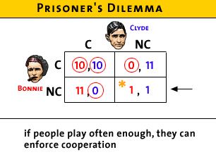
- but if they only play once, the RATIONAL OUTCOME is for
both to confess
- this is rational even if it isn't the best
outcome
- Maybe they can enforce cooperation other ways:
- like through third party enforcement of contracts
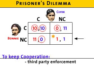
- but more likely, if people play often enough they can
form reputations that they will not cheat; i.e. trust
- Conclusion
- the best outcome may not be individually rational
- it would be better for an individual business to pollute
(cheaper and therefore larger profits), but it would not
best if all businesses polluted
- how to avoid a Nash equilibrium and end up with the best
outcome instead?
- repeated play
- reputation
- contracts
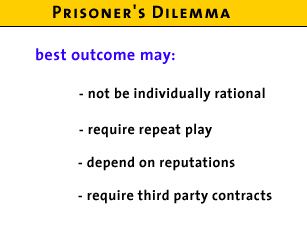
- NOTE: Tomlinson discusses the next lesson when the
prisoners 'dilemma is applied to an oligopoly, I think he is
referring to:
- 10.4-1 Game Theory and Advertising and Brand Names -
Understanding Monopolistic Competition as a Prisoner's Dilemma
AND this should be titled "Understanding Oligopoly as a
Prisoner's Dilemma"
10.4-1 [TW 6.4.3
(6:44)] Game Theory and Advertising and Brand Names -
Understanding Oligopoly (Monopolistic Competition??) as a Prisoner's
Dilemma - 11b
11.2-1
should be done before doing this one
- Outline
- How to use game theory
- Dominant strategy
- Prisoner's Dilemma: Best outcomes vs. Actual
outcomes
- How to use game theory to understand advertising: Coke and
Pepsi
- Assumptions:
- two rivals: Coke and Pepsi competing for a share of the
$10 million soft drink market
- if no advertising they each have $5 million in
sales
- advertising would cost them $3 million
- if you advertise and your rival does not then you get
all customers = $10 million in sales
- if you advertise AND your rival also advertises then you
each get $5 million in sales - the same as if neither
advertise
- Here is the game matrix:
- Coke's Dominant strategy
- The video lecture will ask you a
multiple choice question. ANSWER THE QUESTION by selecting
A, B, or C and more of the lecture will follow
- if Pepsi advertises what ts the
best strategy for COKE?
- if Coke does not advertise it
will get $0 in sales
- if coke does advertise it will
get $2 million in revenue
- BEST for Coke to
advertise
- If Pepsi does NOT advertise, what
is the best strategy for COKE?
- if Coke does not advertise it
will get $5 in sales
- if Coke does advertise it will
get $7 million in revenue
- BEST for Coke to
advertise
- So, Coke has a dominant strategy
to advertise
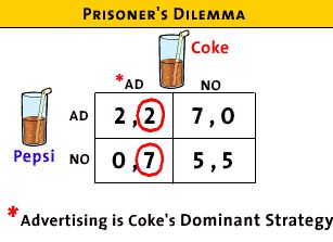
- Pepsi's Dominant strategy
- if Coke advertises what ts the
best strategy for PEPSI?
- if Pepsi does not advertise it
will get $0 in sales
- if Pepsi does advertise it will
get $2 million in revenue
- BEST for Coke to
advertise
- If Coke does NOT advertise, what
is the best strategy for PEPSI?
- if Pepsi does not advertise it
will get $5 in sales
- if Pepsi does advertise it will
get $7 million in revenue
- BEST for Pepsi to
advertise
- So, Pepsi's has a dominant
strategy to advertise
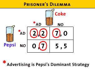
- Best outcomes vs. Actual outcomes
- Best outcome:
- for both Coke and Pepsi is for neither one to advertise
and then they each get $5 million revenue
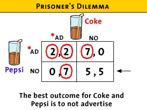
- but this is NOT a self enforcing agreement because they
both will realize that they can now gain by advertising,
- if they agree together that they will not advertise
to achieve their best outcome ($5 million each)
- one can gain if they advertise (i.e. cheat) if the
other one doesn't
- so it makes sense ("individually rational") to cheat
and launch an ad campaign
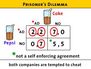
- But the actual outcome (Nash equilibrium) is that they will
both advertise and get only $2 in revenue
- because the best outcome (5,5) is not a self enforcing
agreement
- but if they both advertise, this is a self enforcing
agreement; i.e. they are BOTH giving their best response to
their rival
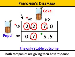
- How to get the best (5,5) outcome:
- they might learn through repeated play that if they both do
not advertise that they will both come out ahead
- or if they can get the government to outlaw soft drink
advertising (they would like and support such a law)
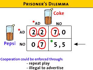
- Prisoner's Dilemma:
- advertising is like the arm's race (nuclear weapons)
- it would be best if no one advertises (or had nuclear
weapons)
- but, because of the possibility of your rival doing it, you
have to keep up
- in the end everyone's profits are reduced (2,2)
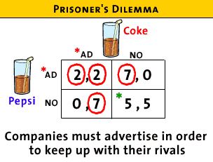
11.3-1 [TW 6.3.2 (10:47)] Understanding a Cartel as a
Prisoner's Dilemma - 11b
- Outline
- Definition of a Cartel
- Prisoner's Dilemma
- Best Outcome
- Definition of a Cartel
- an oligopoly where the individual members try to act as a
monopolist
- ME: (from the textbook) a group of producers that typically
creates a formal written agreement specifying how much each
member will produce and charge. Output must be controlled—the
market must be divided up—in order to maintain the
agreed-upon price. The collusion is overt, or open to
view.
- they get together and act as one, setting the price and
quantity together, choosing the profit maximizing monopoly
quantity and price and earning monopoly profits that they
divide among themselves; i.e. they act as a monopoly
- ME: usually this is done by all member restricting quantity
and raising the price
- Problem: keeping the cartel together is a problem because
of the prisoner's dilemma
- .if one firm knows that all the others are restricting
the quantity which makes the price higher, this firm can
CHEAT and produce more and make greater profits for itself;
i.e. they have an incentive to cheat
- but if all firms or countries) cheat by producing more,
the price will drop and they will all earn lower profits
than if no one cheated
- Prisoner's Dilemma: The Cartel as a case of the Prisoner's
Dilemma
- two countries form an oil cartel, Nigeria and
Venezuela
- they each have two options: cooperate or cheat
- if they both cooperate they earn maximum profits that
are shared ($10 million total or $5 each)
- if both cheat and increase their output then the price
will fall an total profits will fall (to $8 million) and
they will each earn only $4.
- if one cheats and produces more but the other does not
an still produces less, the cheater more profits ($6) ,but
the other makes less profits ($3) and total profits will be
less ($6 + $3 = $9) because the price will be lower; i.e.
they are not earning the highest, monopoly, profit.
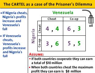
- What are Dominant Strategies?
- For Venezuela:
- if Nigeria cheats, then Venezuela's best response is
to cheat also and profits are 4,4.
- if Nigeria cooperates then Venezuela's best response
is to cheat and profits are 3 for Nigeria and 6 for
Venezuela
- So, Venezuela has an incentive to cheat no matter
what Nigeria does
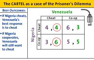
- For Nigeria:
- if Venezuela cheats, then Nigeria's best response is
to cheat also and profits are 4,4.
- if Venezuela cooperates then Nigeria's best response
is to cheat and profits are 3 for Venezuela and 6 for
Venezuela
- So, Nigeria has an incentive to cheat no matter what
Venezuela does
- Nash Equilibrium
- since both countries have a dominant strategy to cheat
the Nash equilibrium is for both top cheat and the cartel
falls apart
- profits are $4 million each
- total profits are at the lowest of all possible
options
- ME: but this is the best outcome for consumers!
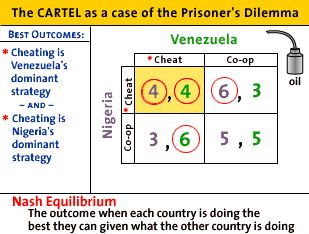
- Best Outcome
- the best outcome for the oil producing countries is to
collude (form the cartel) reduce output, and raise the price
acting like a monopolist
- this way each country would earn profits of $5 million
(5,5)
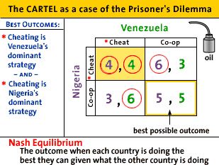
- but this is not a self enforcing agreement because they
each have an incentive to cheat and try to improve their
profits
- so this is not a Nash equilibrium (i.e. not a stable
outcome)
- So, what does this mean about cartels? Are they possible?
Yes, if they learn through
repeated play that cheating hurts them both and that cooperating is
better for them.
[TW 6.3.3 (4:22)] Understanding the Kinked-Demand Curve
Model for $1.98: at: http://mindbites.com/lesson/7742-economics-kinked-demand-curve-model
- 11b
OR TW 6.3.3 Understanding the Kinked-Demand Curve Model
6.3.3
- Outline
- the kinked demand curve
- the discontinuous MR curve
- finding the profit maximizing quantity
- problems with the kinked demand model
- ME: mutual interdependence
- assume:
- that rivals ignore if one firm raises its price
- but rivals will match the price change if one firms decides
to lower its price
- result: the demand curve will be kinked
- it will be more elastic (flatter) above the original price
because if one firm lowers its price AND all of its competitors
do not, then the firm will lose A LOT of customers
- the demand will be less elastic (steeper) below the
original price because if one firm decides to lower its price
all of its competitors will ALSO lower their prices and each
would get only A FEW new customers
- what will the MR curve look like?
- as always (except pure competition) the MR will be below
the demand curve (D)
- it will be discontinuous
- how to find the profit maximizing quantity
- as always, we find the profit maximizing level of output at
the quantity where MR = MC
- It is quite likely that the MC curve will cross the MR
curve in the vertical gap
- if so, then the profit max quantity is found on the
horizontal axis directly below the gap and the price is found
off of the demand curve above
- the price would then be at the kink in the demand
curve
- Problems
- one problem with the model is that it does not tell us how
the kink in the demand curve got where it is in the first
place
- also there are not many good real world examples
- But, logically it does make sense.
Kinked Demand Model
(econclassroom.com 14:06) - 11b
http://www.econclassroom.com/?p=3144
Preview:
- In this lesson we take a graphical approach to oligopoly, and
seek to explain why prices tend not to fluctuate up or down
in oligopolistic markets.
- Why do some oligopolies have very little incentive to decrease
their prices, and also a strong incentive not to raise their
prices?
- What emerges is a kinked demand curve, highly elastic at
prices above the current equilibrium and highly inelastic at
prices below the current equilibrium. Along with this kinked
demand curve comes a kinked marginal revenue curve, with a
vertical section. The implication is that even as an oligopolist's
costs rise and fall in the short-run, its level of output and
price tends to remain stable.
Review - Oligopolies:
- few firms
- mutual interdependence
- Mutual interdependence exists when firms consider their
rivals' reactions while adjusting prices and outputs.
Assumptions about oligopoly
pricing behavior (kinked demand model)
- before changing its price an oligopolist will try to predict
what its competitors will do if they do change their price
- ASSUME: competitors will match price decreases - if one
firm lowers its price the competitors will lower their prices
- This make sense because the competitors will not want to
lose a lot of customers to a competitor that lowers it price,
so they will decrease their price too.
- therefore, the demand curve is inelastic, if all
firms lower their prices they will not gain very many
customers, i.e. the % change is quantity demanded will be small
= inelastic
- ASSUME: competitors ignore price increases - if one
firm raises its price the competitors will not raise their prices
- This makes sense because competitors could gain a lot of
customers if they kept their prices low when one firm raises
theirs
- therefore, the demand curve will be elastic, if one firm
raises its price and the other firms do not, the one firm will
lose a lot of customers, i. e. the % change in quantity
demanded will be large = elastic
So what does the demand curve
look like with these assumption?
- demand below the going price will be inelastic (steeper); a
small increase in quantity if the price is decreased
- demand above the going price will be elastic (flatter); a
large decrease in quantity if the price is increased
- so the demand curve will be "kinked", or bent.
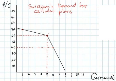
So why are firms reluctant to
change their prices?
- since demand is inelastic below the going price, if a firms
lowers its price (and its competitors do not) then its total
revenues will decrease; a big drop in price but a little increase
in quantity causes TR to decline
- since demand is elastic above the going price, if a firm
raises its price (and all its competitors raise their prices too)
then its total revenues will decrease; a little increase in price
but a large decrease in quantity causes TR to decline
- Therefore, prices in an oligopolistic market are "sticky";
i.e. they tend not to change because if a firms raises, or lowers
its price, its total revenues will fall
So what does the MR curve look
like?
- We know that when the demand curve is downward sloping, the MR
curve is below it
- the MR diminishes at twice the rate that demand does
therefore, we end up with two MR curves, one somewhat flat under
the elastic portion of the kinked demand curve and one more steep
under the inelastic portion of the demand curve, and a vertical
portion of the MR curve connecting the two
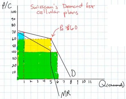
So what will oligopolists do if
their costs change? Will they change their prices and quantities?
- maybe not
- in other markets
- if variable costs rise, the MC will rise and the profit
maximizing level of output (where MR=MC) will decrease,
and
- if variable costs fall, the MC will fall and the profit
maximizing level of output (where MR=MC) will increase
- but in the kinked demand model, if the MC crosses MR in the
vertical section, a change in costs will not change the profit
maximizing level of output or the profit maximizing price. the
price and quantity where MR = MC will stay the same even if MC
rises or falls
ME:
- Most economic textbook and online video lectures do not
include the ATC curve in their kinked demand model. I am not sure
why. And they often include 2 MC curves to show that changes in
costs do not change the profit maximizing quantity or price.
- here is a graph of the oligopoly kinked demand model with the
ATC curve and only one MC:
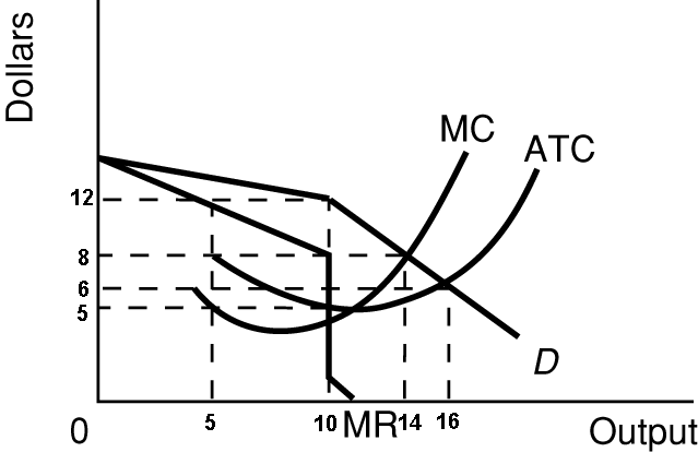
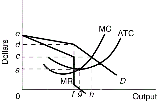
- Profit maximizing quantity and price: Q = f; P = d
- Allocatively efficient quantity and price: Q = h; P =
c
- Productively efficient quantity and price: Q = g; P =
a
Oligopolies, Duopolies,
Collusion, and Cartels (Khan Academy 8:26) - 11b
http://www.khanacademy.org/finance-economics/microeconomics/v/oligopolies--duopolies--collusion--and-cartels
Introduction
- oligopoly
- "oli" means "few"
- "polies" means "sellers"
- sometimes oligopolies act more like monopolies and sometimes
they act more like competitive markets
Collusion (acting more like a
monopoly)
- if they coordinate their pricing and production decisions they
are acting more like a monopoly
- this is called collusion
- this is often illegal
- if they do it formally (like written agreements) then we call
it a cartel
- example of a cartel: OPEC (the Organization of Petroleum
Exporting Countries)
- 12 countries
- control 79% of the world's oil reserve (2012)
- and 44% of the world's oil production (2012)
- attempt to act like a monopoly
- one problem with collusion is that individual firms (or
countries as in OPEC) have an incentive to CHEAT: i.e. they might
be able to make more money if the say that they are going to
charge a high price like the rest of the firms, but then they
lower their price a take customers away from all the other
firms
Oligopolies that are More
Competitive
- Example: Coca-Cola vs.Pepsi
- Coke and Pepsi compete on price and on marketing
- a duopoly is an oligopoly with only two major
firms
- examples of oligopolies that compete (act more like pure
competition):
- Coca-Cola and Pepsi (duopoly)
- Boeing and Airbus (large passenger jet manufacturers -
duopoly)
- Airlines
- most cities have only a few airlines
- their products are very similar (standardized?)
- credit card (Visa, Mastercard, Discover American
Express)
- governments try to assure that oligopolies compete rather than
collude because collusion is inefficient (like monopolies) and
when they compete they are more efficient (more like pure
competition) with a larger consumer plus producer surplus (total
surplus).
SUMMARY
Determining the Efficiency
of Firms in Different Market Structures (econclassroom.com
18:23) - 11b
http://www.econclassroom.com/?p=4456
Introduction
- two types of efficiency
- productive efficiency
- producing at the level of output where its ATC is
minimized
- is the price equal to the minimum ATC
- ME: quantity where MC=ATC
- allocative efficiency
- producing at the level of output where the MB = MC
- achieved where P=MC (or D=MC)
- the demand curve represents the MB that consumers
receive from the consumption of a good
- also called the socially optimal quantity
-
Perfect Competition Long Run
Equilibrium
- very many firms producing standardized (identical) products
with no barriers to entry
- demand perfectly elastic (firm is a price taker) since there
are very many firms producing identical products and no individual
firm has any market power
- D=P=MR
- equilibrium price is established in the market (supply and
demand in the market)
- zero (normal) economic profits in long run equilibrium because
of no barriers to entry so ATC touches demand at the lowest point
of the ATC curve
- quantity produced is where MR=MC (Qpc)
- productive efficiency is achieved
- equilibrium quantity (Qpc) is where ATC is at a minimum
(P=minimum ATC)
- produce the quantity where MC=ATC
- if they produce at any other quantity then the ATC will be
greater than the price and they will earn economic losses and
will go out of business in the long run
- allocatively efficiency is achieved
- at the profit maximizing quantity (Qpc) the P=MC
- MSB=MSC
- this is the socially optimal quantity
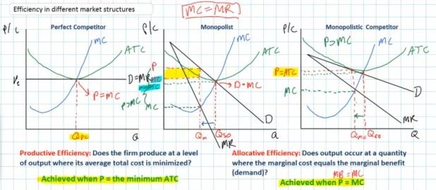
Monopoly Long Run
Equilibrium
- single firm in the industry since entry is blocked
- producing a unique product
- downward sloping demand since the monopolist has market power
since it produces a unique product that no other firms produce and
the demand (or P) is greater then the MR
- D=P>MR
- long run profits likely shown on graph as the ACT is below the
demand (P) curve because entry is blocked (yellow rectangle)
- quantity produced is where MR=MC (Qm)
- productive efficiency is NOT achieved
- equilibrium quantity (Qm) is NOT where ATC is at a minimum
(P>minimum ATC)
- they do NOT produce the quantity where MC=ATC
- at the profit maximizing level of output (Qm) the actual
ATC is higher than the minimum ATC
- since there is no competition the firm does not need to
produce in the least cost manner; without competition the firm
can charge a much higher price and produce at a higher ATC and
earn greater profits
- allocative efficiency is NOT achieved
- equilibrium quantity (Qm) is NOT at the quantity where P=MC
(Qso)
- at the profit maximizing level of output (Qm), P>MC
- meaning that there is an underallocation of resources; too
little is being produced
- monopolists can restrict output to increase the price and
earn greater profits
- at the socially optimal (alloc. eff.) quantity (Qso),
profits are not maximized so the monopolist will not produce
this quantity
Monopolistic Competition Long
Run Equilibrium
- many firms in the industry producing similar products
- some market power (price making power) because of product
differentiation
- downward sloping demand for the individual firms but more
elastic since there are many substitutes and the demand (or P) is
greater then the MR
- D=P>MR
- zero (normal) economic profits in long run equilibrium because
of few barriers to entry so ATC is tangent to the demand
curve
- quantity produced is where MR=MC (Qmc)
- productive efficiency is NOT achieved
- equilibrium quantity (Qmc) is NOT where ATC is at a minimum
(P>minimum ATC)
- they do NOT produce the quantity where MC=,ATC
- at the profit maximizing level of output ATC is higher than
the minimum
- allocative efficiency is NOT achieved
- equilibrium quantity (Qmc) is NOT at the quantity where
P=MC
- at the profit maximizing level of output (Qmc),
P>MC
- meaning that there is an underallocation of resources; too
little is being produced
- as long as firms have some market power (i.e. the demand is
downward sloping) they will maximize profits by producing a
quantity that is less than the socially optimal quantity
(Qso)
Summary
- imperfect competition (monopoly, monopolistic competition, and
oligopoly) is a form of market failure; the market fails to
achieve efficiency as we saw in this lesson
- ME: we studied market failure when we studied externalities in
chapter 5; when externalities exists markets fail to achieve
efficiency
- ME: in chapter 2 where we studied the economic functions of
government, one of the functions was to try to maintain
competition ;i.e. to correct markets when they fail to achieve
efficiency; we also studied this in chapter 18 when we discussed
antitrust laws and monopoly regulation
- since most industries are imperfectly competitive, does this
mean that the most markets are market failures?
- if we just look at the graphs we would have to answer
"yes", "technically speaking"
- but there are also some benefits to imperfectly competitive
markets that also have to be considered:
- the great degree of product differentiation provides
society with a lot of benefits that may make up for some of
the underallocation of resources (customer service,
innovation, product development); variety is good
UNIT 4
Chapter 12 (Module 12a)
MODULE 12a - THE DEMAND FOR RESOURCES
12.1-1 [TW 7.1.1 (15:10)] Deriving the Factor
Demand Curve - 12a
- Outline:
- A firm's demand for a resource like labor is a derived
demand. It is derived from the demand for the product that the
resource produces
- The profit maximizing rule says that a firm hires labor
up to the point at which MRP = MRC (or MRP = W in competitive
labor markets)
- to maximize profits, a firm will keep hiring workers until the
last worker adds just enough revenue to the firm to cover the cost
of that worker
- the demand for labor (by businesses) is a derived
demand, that means it resutls from the demand for the products
that the labor produces
- MRP = change in TR / change in quantity of labor
- MRP = the extra revenue that the firm gets when it hires
one more worker
- MRP = the MB to the firm of hiring another worker
- MRP = MR x MP
- MR = extra output of produding one more unit of
output
- MP = extra output from hirirng one more worker
- for purely competitive product market: MRP = P x MP =
VMP = value of the marginal product
- ME:
- this is just benefit-cost analysis
- they hire all workers where the MB > MC, up to where
the MB = MC
- But, how do we measure the MB of another worker and the
MC of another worker?
- MRP
- marginal revenue product
- the MB that a firm gets when it hires another worker
- Definition: the increase in the firm's total revenue
derived from hiring one additional worker (or any other
variable input
- Formula: MRP = change in TR / change in quantity of
labor
- VMP
- VMP is the Value of the Marginal Output
- VMP is the value (P) of the extra output produce by adding
one more worker (MP)
- VMP = the price of the output (P) times the extra output
produced by the last unit of labor hired (MP)
- P x MP is called the VMP
- if the firm is perfectly competitive then MRP = VMP
- MRP = MR x MP
- but in pure competition we know that MR = P
- so for firm's selling their product in a perfectly
competitve market: MRP = P x MP
- VMP = value of the marginal product = P x MP
- VMP = MRP (for firms in purely competitive product markets
only)
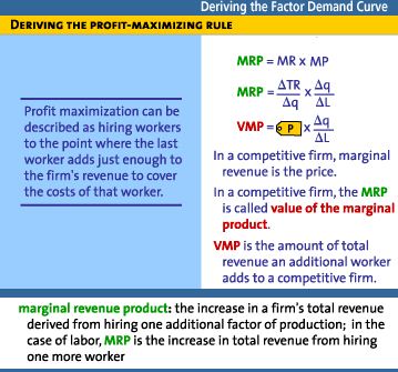
- What is the profit maximizing quantity of labor to hire if the
firm is purely competitive in the short run?
- ME:
- we need to know the extra benefits of hiring one more
worker and the extra costs of hiring one more worker
- then we hire up to the point that MB=MC
- MB of hiring one more worker is the MRP or the amount
that TR increases when we add one more worker
- MC of hring one more worker
- is the MRC
- margnal resource cost
- MRC = change in TC / change in quantity of labor
- so we will maximize profits if we keep hiring as long as
the worker adds more to our revenue (MRP) than it does to
our costs (MRC)
- profit maximizing rule: MRP = MRC
- Given:
- P of TVs = $100
- and the table below
- what is the profit maximizing Q of labor to
hire?
- i.e. where does MRP = MRC, or in purely competitive
product markets, where does VMP = W or MRP = W
- hire as long as the VMP is > wage you have to pay up
to where VMP = W
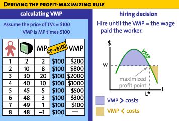
- hire L* number of workers
- thr VMP curve then is the derived demand curve of
labor
- it is also the MRP curve; in purely competitive product
markets VMP = MRP
- So: the demand for labor is the MRP curve
- VMP = P of the product x MP
- MRP = change in TR / change in Q labor
- New rule for maximizing profits in purely competitive
product markets only: W = VMP or W = MRP
- New rule for maximizing profits in purely competitive product
markets: W = VMP or W = MRP
- this is really the same as MR = MC
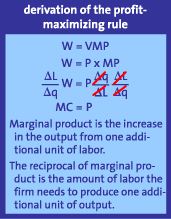
- Now we can draw a Demand curve for Labor
- Remember: DEMAND is a schedule that shows the quantiy
employed at various wages
- we know they will hire the quantity up to where the W = MRP
(or until W = VMP in purely competitive product markets)
- so we can pick different wages and find the quantity of
labor demanded at each wage
- ME:
- the VMP = W rule is only good if BOTH the product market
AND the labor markewt are purely competitive
- a more general rule to maximize profits is: MRP =
MRC
- also, our textbook only shows the MRP (or VMP here) to
be downward sloping, just to keep it simple
- SO, the MRP curve (or VMP here with purely
competitive product ASD resource markets) is the resource
demand curve
- What will change (shift) the demand for labor (resource)?
- anything that changes the demand for thr product (P, P, I,
N, T)
- anything that changes the productivity of the resource
(like technology)
- ME: also, changes in the prices of other resources (but
this is complicated -- see textbook)
- ME: see the textbook for a more in depth discussion of the
determinants of resource (labor) demand
- What happens if you do not have a purely competitve product
market and firms have to lower their prices to sell more?
- then VMP will not be the same as MRP
- to find the profit maximizing quantity to hire: MRP = W (or
VMP = W)
- ME:
- but this is only if the RESOURCE market is
competitive
- a more general rule is: to maximize profits hire labor
up to the point where MRP = MRC
- SUMMARY:
- ALWAYS to find the profit maximizing quantity to hire:
MRP = MRC
- ONLY WITH competitive product AND resource markets: VMP
= W
- ONE MORE THING: since we know compeititve markets are
efficient, then the qallocatively efficient quantity to hire is
where: VMP = W
12.3-1 [TW 7.1.3 (15:24)] The Supply of Labor -
The Determination of Wages - Analyzing the Labor Market - 12a
- Outline:
- Demand for Labor = MRP
- individual demand
- market demand: horizontal summation
- Supply of Labor
- Equilibrium in the Labor Market
- Demand for labor is the firm's MRP curve
- For ALL graphs in econmics you should be able to answer
three questions:
- what is the relationship being described by the graph?
- what accounts for the slope, or shape, of the curve?
- what would cause the curve to shift?
- for the MRP curve:
- the relationship is the relationship between the wage in th
emarket and the quantity of labor than an individual firm finds
profitable to hire
- the MRP curve is downward sloping because of the
diminishing MP of labor; that is, since each additional workers
produce less additinal output than the previous worker so they
therefore add less to the firm's revenue
- if the MP of labor declines rapidly the demand for labor
(MRP) will be more elastic and a small change in the wage
rate will cause a large change in the quantity hired
- ME: the textbook gives the folowinf determinants of
elasticity of demand for labor:
- rate of MP decline
- ease of resource substitutability
- elasticity of product demand
- labor-cost to total-cost ratio
- the demand for labor will shift in responsese to changes in
two determinants:
- a change in the price of the good or sevice being
produced
- a change in labor productivity
- Market Demand: horizontal summation
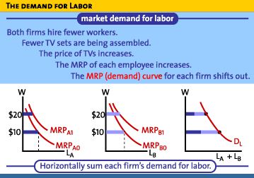
- The Supply curve for labor
- individual households supply labor to businesses
- how much labor will people be willing to supply at
different wages
- tradeoff between work or leisure?
- a backward bending supply of labor curve?
- if wages are high people might decide to work less and
take more leisure - called the income affect
- but the substitutin effect says that if wages are high
people might work more and take less leisure
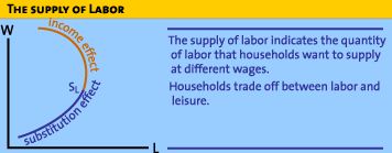
- but usually econmists assume an upward sloping l;abor
supply curve:
- what relationship: the relationship the market wage and
rthe amount of time people want to spend at work
- why the upward slope: because the higher the market wage
the more people want to work
- whar causes the curve to shift: examples:
- lower taxes so people get to keep more of their
income
- if people needed more income like for medical
bills
- if preferences toward work and leisure changed
- Equilbrium
- where the labor D and S cross
- Qs = Qd is equilibrium; why
- if wages are too low then the Qd>Qs and there will be
a shortage of labor or excess demand for labore will bid
wages up through the bidding mechanism
- if wages are too high the the Qd<Qs and there will be
excess supply and the bidding mechanism will drive wages
lower
- shifts in the demand or supply of labor graphs will change
the equilibrium wage rate and the quantity employed
(THE LOST EPISODES) Factor Market Overview (YouTube mjmfoodle
1:27) -12a
http://www.youtube.com/watch?v=J0LigIdph8I&list=UU_xHLAJ_zqPHkmC2aY2MdcA
(The Lost Episodes) Perfectly Competitive Factor and Output
Markets 5:14) -12a
http://www.youtube.com/watch?v=OUyvqq6ZY6s&list=UU_xHLAJ_zqPHkmC2aY2MdcA&index=2
Chapter 13 Wage Determination (Module 13a)
MODULE 13a WAGE DETERMINATION (LABOR
MARKETS)
Chapter 20 (Module 20a)
MODULE 20a - INCOME INEQUALITY AND
DISCRIMINATION
13.3-1 [TW10.3.4 (5:20)] Income Distribution in
the U.S. and the Poverty Level - 20a
- Outline:
- Income Distribution
- Poverty
- Income Distribution
- median income in the US in 2004 was $43,389
- ME: "median" means that half the families earned less
ans half earned more
- doesn't tell ust how the incme is distributed
- do most families earn about $43,00
- or do some earn a lot more ans others a lot
less?
- Distribution by quintiles:
- Changes over time:
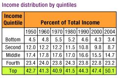
- little change from 1950-1990
- 1990: top quintile begins to earn a greater share of all
income
- 2000: bottom quintile begins to earn a smaller share of
all income
- Poverty Level (2004)
- poverty level

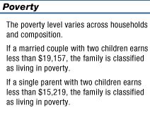
- poverty rate:
- the % of families with invcomes below the poverty
level
- 2004: 12.7% of families in the US were living in poverty
(about 1/8)
- the poverty rate used to be much higher
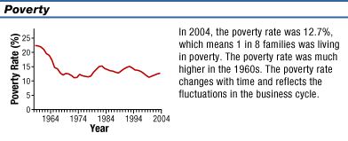
- poverty rates differ for different demographic groups
- white families have lower rates than minorities
- single mother headed households have higher
rates
- which families living in poverty CHANGES a lot
- in any 10 year period, 4 families out of 10 will at
some time be lining in pocerty in the united States
- less than 3% od families live in poverty for long
periods of time
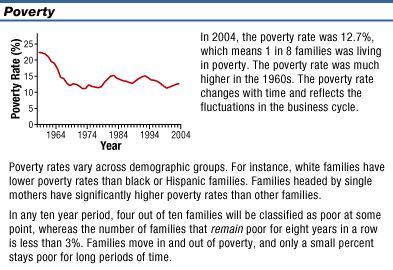
- What can be done?
- progressive income taxes help the government pay for:
- transfer payments
- in-kind transfers
- public goods
- provide opportunities for acquiring human and financial
capital
- Incentive effects of poverty programs
Chapter 22 (Module 22a)
MODULE 22a - IMMIGRATION
OPTIONAL: