Start Up: Crazy for Coffee
Starbucks Coffee Company revolutionized the coffee-drinking habits
of millions of Americans. Starbucks, whose bright green-and-white
logo is almost as familiar as the golden arches of McDonald's, began
in Seattle in 1971. Fifteen years later it had grown into a chain of
four stores in the Seattle area. Then in 1987 Howard Schultz, a
former Starbucks employee, who had become enamored with the culture
of Italian coffee bars during a trip to Italy, bought the company
from its founders for $3.8 million. In 2008, Americans were willingly
paying $3 or more for a cappuccino or a latte, and Starbuck's had
grown to become an international chain, with over 16,000 stores
around the world.
The change in American consumer's taste for coffee and the profits
raked in by Starbucks lured other companies to get into the game.
Retailers such as Seattle's Best Coffee and Gloria Jean's Coffees
entered the market, and today there are thousands of coffee bars,
carts, drive-throughs, and kiosks in downtowns, malls, and airports
all around the country. Even McDonald's began selling specialty
coffees.
But over the last decade the price of coffee beans has been quite
volatile. Just as consumers were growing accustomed to their
cappuccinos and lattes, in 1997, the price of coffee beans shot up.
Excessive rain and labor strikes in coffee-growing areas of South
America had reduced the supply of coffee, leading to a rise in its
price. In the early 2000s, Vietnam flooded the market with coffee,
and the price of coffee beans plummeted. More recently, weather
conditions in various coffee-growing countries reduced supply, and
the price of coffee beans went back up.
Markets, the institutions that bring together buyers and
sellers, are always responding to events, such as bad harvests and
changing consumer tastes that affect the prices and quantities of
particular goods. The demand for some goods increases, while the
demand for others decreases. The supply of some goods rises, while
the supply of others falls. As such events unfold, prices adjust to
keep markets in balance. This chapter explains how the market forces
of demand and supply interact to determine equilibrium prices and
equilibrium quantities of goods and services. We will see how prices
and quantities adjust to changes in demand and supply and how changes
in prices serve as signals to buyers and sellers.
The model of demand and supply that we shall develop in this
chapter is one of the most powerful tools in all of economic
analysis. You will be using it throughout your study of economics. We
will first look at the variables that influence demand. Then we will
turn to supply, and finally we will put demand and supply together to
explore how the model of demand and supply operates. As we examine
the model, bear in mind that demand is a representation of the
behavior of buyers and that supply is a representation of the
behavior of sellers. Buyers may be consumers purchasing groceries or
producers purchasing iron ore to make steel. Sellers may be firms
selling cars or households selling their labor services. We shall see
that the ideas of demand and supply apply, whatever the identity of
the buyers or sellers and whatever the good or service being
exchanged in the market. In this chapter, we shall focus on buyers
and sellers of goods and services.
3a Demand

If the
price of pizza goes up, what happens to the demand for pizza? . .
. . . . . . . . . . . . . . . . . NOTHING! Nothing happens to the
demand for pizza if the price changes!
The next three
lessons introduce the demand and supply model for explaining how
prices arise and change in a market economy. Learn these lessons
well. Do the assigned problems. Draw the graphs in the yellow
pages and while you are reading and studying. DRAW GRAPHS! Get
used to using the graphs to help you answer questions. If you are
avoiding drawing the graphs you will do poorly and not get the
practice that you need to learn the concept. Be sure to LABEL the
axes of every graph that you draw.
So why doesn't
the demand for pizza change if the price changes? Because
economists have a different definition of "demand". Demand is NOT
the quantity that we buy. If the price of pizza goes up we will
buy less, but that is not what "demand" means in economics.
Economists tend to be precise with their definitions and sometimes
their definitions are different than the more commonly used
definitions. Things like "scarcity", "investment", "cost",
"demand", and "supply", have different definitions in economics
than what you may already know. Learn our definitions! Demand is
not how much we buy. Demand has a different definition in
economics. "Demand" means the "demand graph".
Remember, that
econmists use models (like the supply and demand model) to
simplify the real world. They do this by isolating certain
variables from all the clutter found in reality. Then by changing
one variable at a time economists can see what effect it will
have. In this lesson we will learn the economic definition of
DEMAND and plot the demand graph. Then, we will look at one
variable at a time to see what effect they have on the demand
curve. We call these variables the "non-price determinants of
demand". They are: Pe, Pog, I, Npot, T (P,P,I,N,T). LEARN THEM!
LEARN THEM WELL! Know how each one affects the demand curve. Be
sure to do the yellow pages.

What is
that Campbell's Pork and Beans can doing on the display for
VanCamp's Pork and Beans (see below)?
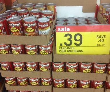
After studying
this lesson you will be able to draw a graph illustrating what
happened to the demand for Campbell's Pork and Beans when a
customer took a can out of their shopping cart and placed it on
this display of VanCamp's Pork and Beans that were on sale.
We will learn
which non-price determinant of demand explains why that
Campbell's soup can is there?

TOPICS
- Definition of demand
- Changes in Demand vs. Changes in Quantity Demanded
- Non-price determinants of demand and how they affect
the demand curve
OUTCOMES
- define demand (note: it has a DIFFERENT DEFINITION in
economics)
- If the price of pizza goes up, why does the demand for
pizza stay the same?
- be able to correctly draw and label a demand graph
- why do economists employ the ceteris paribus assumption
when creating a demand curve?
- what is the law of demand?
- why is the demand curve downward sloping (three
explanations)
- list the non-price determinants of demand (Pe. Pog, I,
Npot, T) or (P, P, I, N, T ) and understand how they affect the
demand schedule and curve. This is VERY IMPORTANT. BE ABLE TO
DO THIS! See the 3a/3b/3c yellow pages.
- explain the difference between the a "change in the
quantity demanded" and a "change in demand"
- what is an "increase in demand" and a "decrease in demand"
and show how they affect the demand schedule and the demand
curve
- what is "market demand"?
- what is that Campbell's Pork and Beans can doing on the
display for VanCamp's Pork and Beans (see picture at left)?
Which non-price determinant of demand explains why that
Campbell's soup can is there? Draw a supply and demand graph
illustrating what happened in the market for Campbell's Pork
and Beans when VanCamp's were put on sale.

Key
Terms Flash Cards - Click Here
demand,
quantity demanded, law of demand, market demand, horizontal
summation, income effect, substitution effect, diminishing
marginal utility, change in demand, change in quantity demanded,
increase in demand, decrease in demand, non-price determinants of
demand, normal good, inferior good, substitute good, complementary
good (complement), independent goods

How many
pizzas will people eat this year? How many doctor visits will people
make? How many houses will people buy?
Each
good or service has its own special characteristics that determine
the quantity people are willing and able to consume. One is the price
of the good or service itself. Other independent variables that are
important determinants of demand include consumer preferences, prices
of related goods and services, income, demographic characteristics
such as population size, and buyer expectations. The number of pizzas
people will purchase, for example, depends very much on whether they
like pizza. It also depends on the prices for alternatives such as
hamburgers or spaghetti. The number of doctor visits is likely to
vary with income�people with higher incomes are likely
to see a doctor more often than people with lower incomes. The
demands for pizza, for doctor visits, and for housing are certainly
affected by the age distribution of the population and its size.
While
different variables play different roles in influencing the demands
for different goods and services, economists pay special attention to
one: the price of the good or service. Given the values of all the
other variables that affect demand, a higher price tends to reduce
the quantity people demand, and a lower price tends to increase it. A
medium pizza typically sells for $5 to $10. Suppose the price were
$30. Chances are, you would buy fewer pizzas at that price than you
do now. Suppose pizzas typically sold for $2 each. At that price,
people would be likely to buy more pizzas than they do now.
We will
discuss first how price affects the quantity demanded of a good or
service and then how other variables affect demand.
Price and the Demand Curve
Because
people will purchase different quantities of a good or service at
different prices, economists must be careful when speaking of the
�demand� for something. They have therefore
developed some specific terms for expressing the general concept of
demand.
The quantity
demanded of a good or service is the quantity buyers are
willing and able to buy at a particular price during a particular
period, all other things unchanged. (As we learned, we can substitute
the Latin phrase �ceteris paribus� for
�all other things unchanged.�) Suppose, for
example, that 100,000 movie tickets are sold each month in a
particular town at a price of $8 per ticket. That
quantity�100,000�is the quantity of movie
admissions demanded per month at a price of $8. If the price were
$12, we would expect the quantity demanded to be less. If it were $4,
we would expect the quantity demanded to be greater. The quantity
demanded at each price would be different if other things that might
affect it, such as the population of the town, were to change. That
is why we add the qualifier that other things have not changed to the
definition of quantity demanded.
A demand
schedule is a table that shows the quantities of a good or
service demanded at different prices during a particular period, all
other things unchanged. To introduce the concept of a demand
schedule, let us consider the demand for coffee in the United States.
We will ignore differences among types of coffee beans and roasts,
and speak simply of coffee. The table in Figure
3.1 �A Demand Schedule and a Demand Curve�
shows quantities of coffee that will be demanded each month at prices
ranging from $9 to $4 per pound; the table is a demand schedule. We
see that the higher the price, the lower the quantity demanded.
The
information given in a demand schedule can be presented with a demand
curve, which is a graphical representation of a demand
schedule. A demand curve thus shows the relationship between the
price and quantity demanded of a good or service during a particular
period, all other things unchanged. The demand curve in Figure
3.1 �A Demand Schedule and a Demand Curve�
shows the prices and quantities of coffee demanded that are given in
the demand schedule. At point A, for example, we see that 25 million
pounds of coffee per month are demanded at a price of $6 per pound.
By convention, economists graph price on the vertical axis and
quantity on the horizontal axis.
Price
alone does not determine the quantity of coffee or any other good
that people buy. To isolate the effect of changes in price on the
quantity of a good or service demanded, however, we show the quantity
demanded at each price, assuming that those other variables remain
unchanged. We do the same thing in drawing a graph of the
relationship between any two variables; we assume that the values of
other variables that may affect the variables shown in the graph
(such as income or population) remain unchanged for the period under
consideration.
A
change in price, with no change in any of the other variables that
affect demand, results in a movement along the demand curve.
For example, if the price of coffee falls from $6 to $5 per pound,
consumption rises from 25 million pounds to 30 million pounds per
month. That is a movement from point A to point B along the demand
curve in Figure
3.1 �A Demand Schedule and a Demand Curve�.
A movement along a demand curve that results from a change in price
is called a change
in quantity demanded. Note that a change in quantity demanded
is not a change or shift in the demand curve; it is a movement
along the demand curve.
The
negative slope of the demand curve in Figure
3.1 �A Demand Schedule and a Demand Curve�
suggests a key behavioral relationship of economics. All other things
unchanged, the law
of demand holds that, for virtually all goods and services, a
higher price leads to a reduction in quantity demanded and a lower
price leads to an increase in quantity demanded.
The
law of demand is called a law because the results of countless
studies are consistent with it. Undoubtedly, you have observed one
manifestation of the law. When a store finds itself with an overstock
of some item, such as running shoes or tomatoes, and needs to sell
these items quickly, what does it do? It typically has a sale,
expecting that a lower price will increase the quantity demanded. In
general, we expect the law of demand to hold. Given the values of
other variables that influence demand, a higher price reduces the
quantity demanded. A lower price increases the quantity demanded.
Demand curves, in short, slope downward.
Changes in Demand
Of
course, price alone does not determine the quantity of a good or
service that people consume. Coffee consumption, for example, will be
affected by such variables as income and population. Preferences also
play a role. The story at the beginning of the chapter illustrates as
much. Starbucks �turned people on� to coffee. We
also expect other prices to affect coffee consumption. People often
eat doughnuts or bagels with their coffee, so a reduction in the
price of doughnuts or bagels might induce people to drink more
coffee. An alternative to coffee is tea, so a reduction in the price
of tea might result in the consumption of more tea and less coffee.
Thus, a change in any one of the variables held constant in
constructing a demand schedule will change the quantities demanded at
each price. The result will be a shift in the entire demand
curve rather than a movement along the demand curve. A shift
in a demand curve is called a change
in demand.
Suppose,
for example, that something happens to increase the quantity of
coffee demanded at each price. Several events could produce such a
change: an increase in incomes, an increase in population, or an
increase in the price of tea would each be likely to increase the
quantity of coffee demanded at each price. Any such change produces a
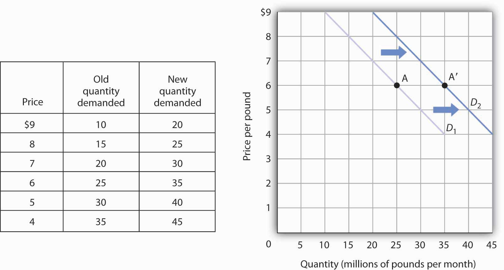
new demand schedule. Figure
3.2 �An Increase in Demand� shows such a
change in the demand schedule for coffee. We see that the quantity of
coffee demanded per month is greater at each price than before. We
show that graphically as a shift in the demand curve. The original
curve, labeled D1, shifts to the right to
D2. At a price of $6 per pound, for example, the
quantity demanded rises from 25 million pounds per month (point A) to
35 million pounds per month (point A�).
Just
as demand can increase, it can decrease. In the case of coffee,
demand might fall as a result of events such as a reduction in
population, a reduction in the price of tea, or a change in
preferences. For example, a definitive finding that the caffeine in
coffee contributes to heart disease, which is currently being debated
in the scientific community, could change preferences and reduce the
demand for coffee.
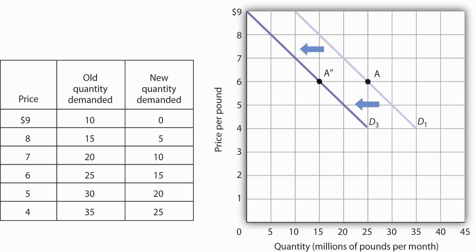
A
reduction in the demand for coffee is illustrated in Figure
3.3 �A Reduction in Demand�. The demand
schedule shows that less coffee is demanded at each price than in
Figure
3.1 �A Demand Schedule and a Demand Curve�.
The result is a shift in demand from the original curve
D1 to D3. The quantity of
coffee demanded at a price of $6 per pound falls from 25 million
pounds per month (point A) to 15 million pounds per month (point
A�). Note, again, that a change in quantity demanded,
ceteris paribus, refers to a movement along the demand
curve, while a change in demand refers to a shift in the
demand curve.
A
variable that can change the quantity of a good or service demanded
at each price is called a demand
shifter. When these other variables change, the
all-other-things-unchanged conditions behind the original demand
curve no longer hold. Although different goods and services will have
different demand shifters, the demand shifters are likely to include
(1) consumer preferences, (2) the prices of related goods and
services, (3) income, (4) demographic characteristics, and (5) buyer
expectations. Next we look at each of these.
Preferences
Changes
in preferences of buyers can have important consequences for demand.
We have already seen how Starbucks supposedly increased the demand
for coffee. Another example is reduced demand for cigarettes caused
by concern about the effect of smoking on health. A change in
preferences that makes one good or service more popular will shift
the demand curve to the right. A change that makes it less popular
will shift the demand curve to the left.
Prices of Related Goods and
Services
Suppose
the price of doughnuts were to fall. Many people who drink coffee
enjoy dunking doughnuts in their coffee; the lower price of doughnuts
might therefore increase the demand for coffee, shifting the demand
curve for coffee to the right. A lower price for tea, however, would
be likely to reduce coffee demand, shifting the demand curve for
coffee to the left.
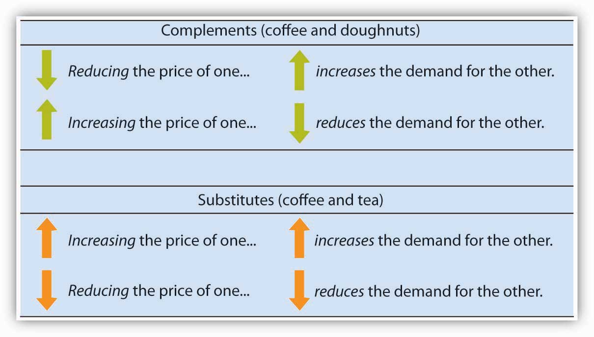
In
general, if a reduction in the price of one good increases the demand
for another, the two goods are called complements.
If a reduction in the price of one good reduces the demand for
another, the two goods are called substitutes.
These definitions hold in reverse as well: two goods are complements
if an increase in the price of one reduces the demand for the other,
and they are substitutes if an increase in the price of one increases
the demand for the other. Doughnuts and coffee are complements; tea
and coffee are substitutes.
Complementary
goods are goods used in conjunction with one another. Tennis rackets
and tennis balls, eggs and bacon, and stationery and postage stamps
are complementary goods. Substitute goods are goods used instead of
one another. iPODs, for example, are likely to be substitutes for CD
players. Breakfast cereal is a substitute for eggs. A file attachment
to an e-mail is a substitute for both a fax machine and postage
stamps.
Income
As
incomes rise, people increase their consumption of many goods and
services, and as incomes fall, their consumption of these goods and
services falls. For example, an increase in income is likely to raise
the demand for gasoline, ski trips, new cars, and jewelry. There are,
however, goods and services for which consumption falls as income
rises�and rises as income falls. As incomes rise, for
example, people tend to consume more fresh fruit but less canned
fruit.
A
good for which demand increases when income increases is called a normal
good. A good for which demand decreases when income increases
is called an inferior
good. An increase in income shifts the demand curve for fresh
fruit (a normal good) to the right; it shifts the demand curve for
canned fruit (an inferior good) to the left.
Demographic Characteristics
The
number of buyers affects the total quantity of a good or service that
will be bought; in general, the greater the population, the greater
the demand. Other demographic characteristics can affect demand as
well. As the share of the population over age 65 increases, the
demand for medical services, ocean cruises, and motor homes
increases. The birth rate in the United States fell sharply between
1955 and 1975 but has gradually increased since then. That increase
has raised the demand for such things as infant supplies, elementary
school teachers, soccer coaches, in-line skates, and college
education. Demand can thus shift as a result of changes in both the
number and characteristics of buyers.
Buyer Expectations
The
consumption of goods that can be easily stored, or whose consumption
can be postponed, is strongly affected by buyer expectations. The
expectation of newer TV technologies, such as high-definition TV,
could slow down sales of regular TVs. If people expect gasoline
prices to rise tomorrow, they will fill up their tanks today to try
to beat the price increase. The same will be true for goods such as
automobiles and washing machines: an expectation of higher prices in
the future will lead to more purchases today. If the price of a good
is expected to fall, however, people are likely to reduce their
purchases today and await tomorrow�s lower prices. The
expectation that computer prices will fall, for example, can reduce
current demand.
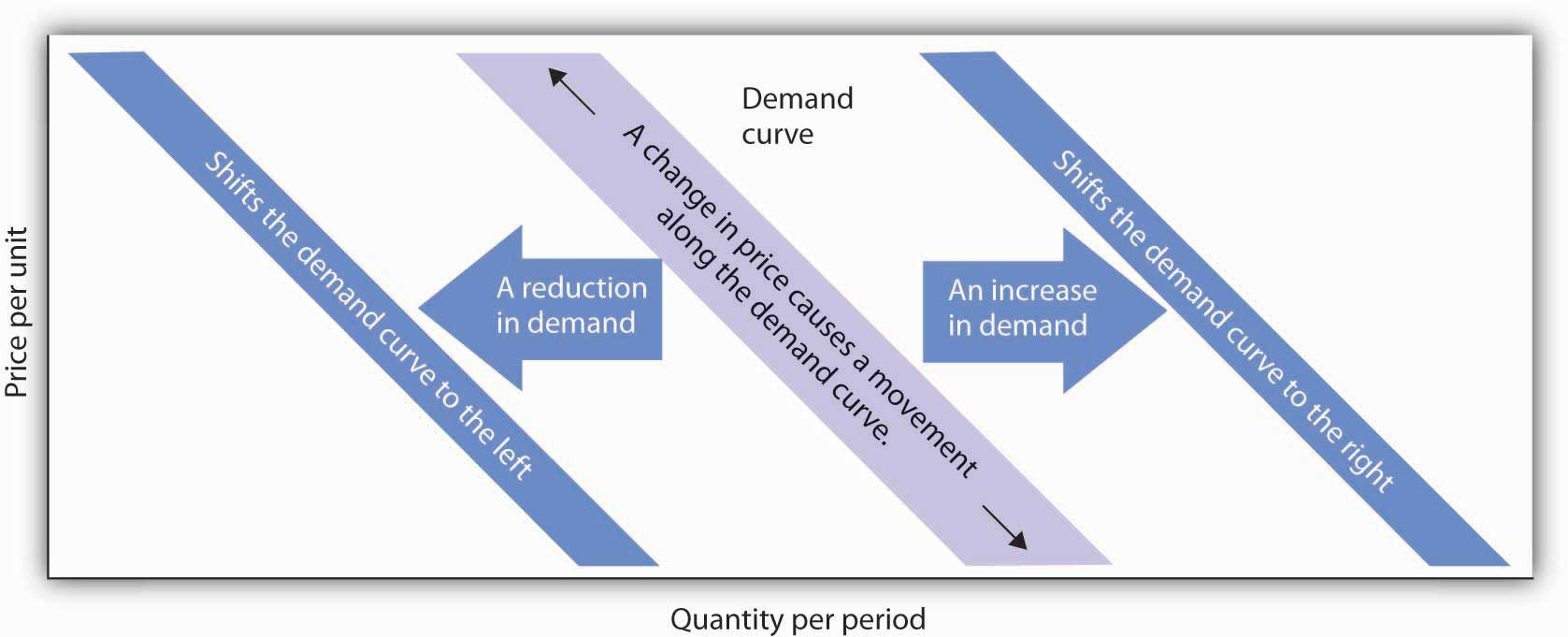
Heads Up!
It is crucial to
distinguish between a change in quantity demanded, which is a
movement along the demand curve caused by a change in price, and a
change in demand, which implies a shift of the demand curve itself. A
change in demand is caused by a change in a demand shifter. An
increase in demand is a shift of the demand curve to the right. A
decrease in demand is a shift in the demand curve to the left. This
drawing of a demand curve highlights the difference.
Key Takeaways
- The quantity demanded of a good or service is the quantity
buyers are willing and able to buy at a particular price during a
particular period, all other things unchanged.
- A demand schedule is a table that shows the quantities of a
good or service demanded at different prices during a particular
period, all other things unchanged.
- A demand curve shows graphically the quantities of a good or
service demanded at different prices during a particular period,
all other things unchanged.
- All other things unchanged, the law of demand holds that, for
virtually all goods and services, a higher price induces a
reduction in quantity demanded and a lower price induces an
increase in quantity demanded.
- A change in the price of a good or service causes a change in
the quantity demanded�a movement along the
demand curve.
- A change in a demand shifter causes a change in demand, which
is shown as a shift of the demand curve. Demand shifters
include preferences, the prices of related goods and services,
income, demographic characteristics, and buyer expectations.
- Two goods are substitutes if an increase in the price of one
causes an increase in the demand for the other. Two goods are
complements if an increase in the price of one causes a decrease
in the demand for the other.
- A good is a normal good if an increase in income causes an
increase in demand. A good is an inferior good if an increase in
income causes a decrease in demand.
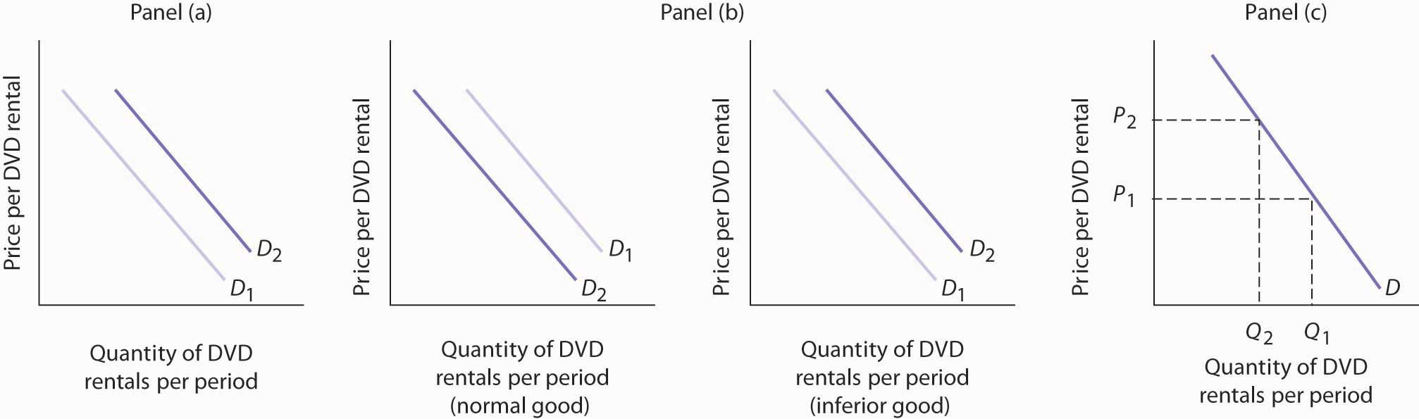
Try It!
All other things
unchanged, what happens to the demand curve for DVD rentals if there
is (a) an increase in the price of movie theater tickets, (b) a
decrease in family income, or (c) an increase in the price of DVD
rentals? In answering this and other �Try It!�
problems in this chapter, draw and carefully label a set of axes. On
the horizontal axis of your graph, show the quantity of DVD rentals.
It is necessary to specify the time period to which your quantity
pertains (e.g., �per period,� �per
week,� or �per year�). On the vertical
axis show the price per DVD rental. Since you do not have specific
data on prices and quantities demanded, make a
�free-hand� drawing of the curve or curves you
are asked to examine. Focus on the general shape and position of the
curve(s) before and after events occur. Draw new curve(s) to show
what happens in each of the circumstances given. The curves could
shift to the left or to the right, or stay where they are.
Case in Point: Solving Campus Parking Problems
Without Adding More Parking Spaces
Unless you attend
a �virtual� campus, chances are you have engaged
in more than one conversation about how hard it is to find a place to
park on campus. Indeed, according to Clark Kerr, a former president
of the University of California system, a university is best
understood as a group of people �held together by a
common grievance over parking.�
Clearly, the
demand for campus parking spaces has grown substantially over the
past few decades. In surveys conducted by Daniel Kenney, Ricardo
Dumont, and Ginger Kenney, who work for the campus design company
Sasaki and Associates, it was found that 7 out of 10 students own
their own cars. They have interviewed �many students who
confessed to driving from their dormitories to classes that were a
five-minute walk away,� and they argue that the deterioration
of college environments is largely attributable to the increased use
of cars on campus and that colleges could better service their
missions by not adding more parking spaces.
Since few
universities charge enough for parking to even cover the cost of
building and maintaining parking lots, the rest is paid for by all
students as part of tuition. Their research shows that
�for every 1,000 parking spaces, the median institution
loses almost $400,000 a year for surface parking, and more than
$1,200,000 for structural parking.� Fear of a backlash from
students and their parents, as well as from faculty and staff, seems
to explain why campus administrators do not simply raise the price of
parking on campus.
While Kenney and
his colleagues do advocate raising parking fees, if not all at once
then over time, they also suggest some subtler, and perhaps
politically more palatable, measures�in particular,
shifting the demand for parking spaces to the left by lowering the
prices of substitutes.
Two examples they
noted were at the University of Washington and the University of
Colorado at Boulder. At the University of Washington, car poolers may
park for free. This innovation has reduced purchases of
single-occupancy parking permits by 32% over a decade. According to
University of Washington assistant director of transportation
services Peter Dewey, �Without vigorously managing our
parking and providing commuter alternatives, the university would
have been faced with adding approximately 3,600 parking spaces, at a
cost of over $100 million�The university has created
opportunities to make capital investments in buildings supporting
education instead of structures for cars.� At the University
of Colorado, free public transit has increased use of buses and light
rail from 300,000 to 2 million trips per year over the last decade.
The increased use of mass transit has allowed the university to avoid
constructing nearly 2,000 parking spaces, which has saved about $3.6
million annually.
Sources: Daniel R. Kenney, �How to Solve
Campus Parking Problems Without Adding More Parking,� The
Chronicle of Higher Education, March 26, 2004, Section B, pp.
B22-B23.
Answer to Try It! Problem
Since going to
the movies is a substitute for watching a DVD at home, an increase in
the price of going to the movies should cause more people to switch
from going to the movies to staying at home and renting DVDs. Thus,
the demand curve for DVD rentals will shift to the right when the
price of movie theater tickets increases [Panel (a)].
A decrease in
family income will cause the demand curve to shift to the left if DVD
rentals are a normal good but to the right if DVD rentals are an
inferior good. The latter may be the case for some families, since
staying at home and watching DVDs is a cheaper form of entertainment
than taking the family to the movies. For most others, however, DVD
rentals are probably a normal good [Panel (b)].
An increase in
the price of DVD rentals does not shift the demand curve for DVD
rentals at all; rather, an increase in price, say from
P1 to P2, is a movement
upward to the left along the demand curve. At a higher price, people
will rent fewer DVDs, say Q2 instead of
Q1, ceteris paribus [Panel (c)].
This is a derivative of Principles of
Economics by a publisher who has requested that they and the
original author not receive attribution, which was originally
released and is used under CC BY-NC-SA. This work, unless otherwise
expressly stated, is licensed under a Creative
Commons Attribution-NonCommercial-ShareAlike 4.0 International
License.
 Microeconomics