![]()
|
UNIT 1: Introduction to
Microeconomics
|
UNIT 3: Product Markets and
Efficiency
|
|
UNIT 2: Elasticity, Consumer Choice,
and Costs
|
UNIT 4: Resource Markets, Inequality,
and Immigration
|
![]()
|
1a Day One- An Introduction to ECO 211 |
Welcome to ECO 211! My name is Mark Healy. I will be your economics instructor for the semester. Please call me "Mark". Many students end up dropping or failing this course due to the lack of basic math skills. If your math skills are weak you should consider building them before taking this course. If you are required to take MTH 060 or MTH 082 and have not yet done so, do not take this economics course until you have successfully completed one of them. The face-to-face sections will take a practice math quiz on the first day of class. For the online section I have posted the math quiz on our Blackboard site. Take the math quiz on Blackboard or in class. If you score less than 14 or 15, consider dropping ECO 211 and taking a math class first. |
1a Something Interesting - Why are we studying this? |
Optional: a funny look at some major ideas of economics by the "Stand-up Economist". |
1a Assignments: Readings |
Syllabus On-Campus / Syllabus Online |
1a Assignments: Video Lectures |
OPTIONAL: YouTube: Principles of economics, translated by Yoram Bauman |
1a Outcomes - What you should know |
|
1a Key Terms |
Key Terms Flash Cards - Click Here The Class: Required Activity, Yellow Pages, Tomlinson Videos on Thinkwell, Video Notes, LESSONS webpage, Pre-quiz, Clicker Quiz, Practice Exercises, The Math: horizontal (x) axis, vertical (y) axis, origin, direct (positive) relationship, inverse (negative) relationship, slope of a line, positive slope, negative slope, marginal |
1a Formulas |
Slope = rise/run Slope = vertical change / horizontal change Slope = marginal value of the total |
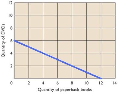
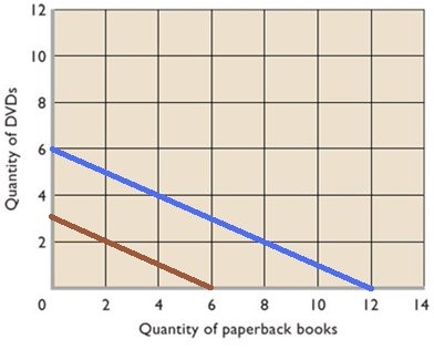
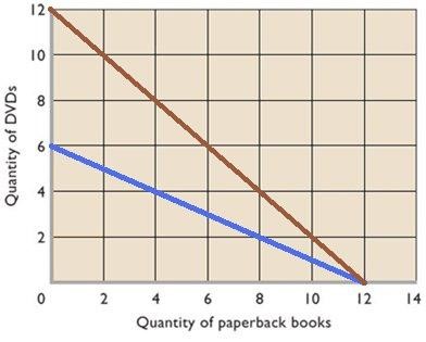
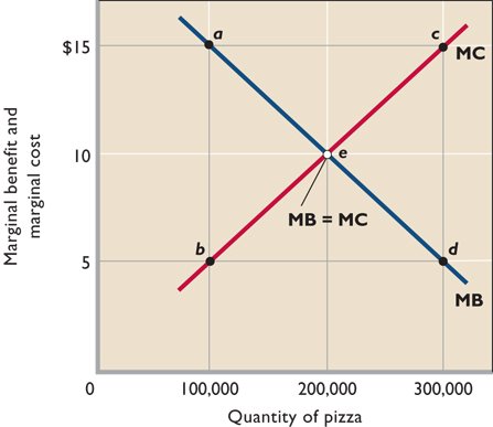
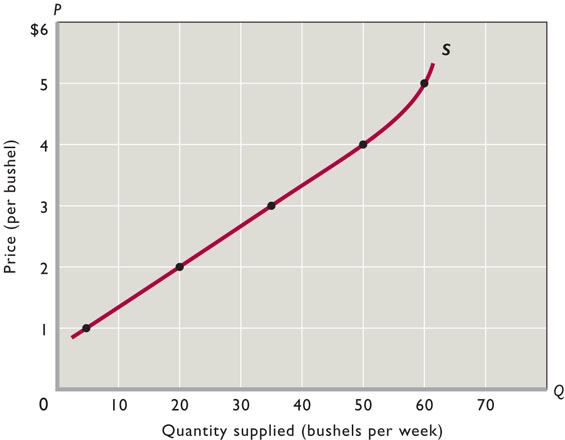
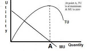
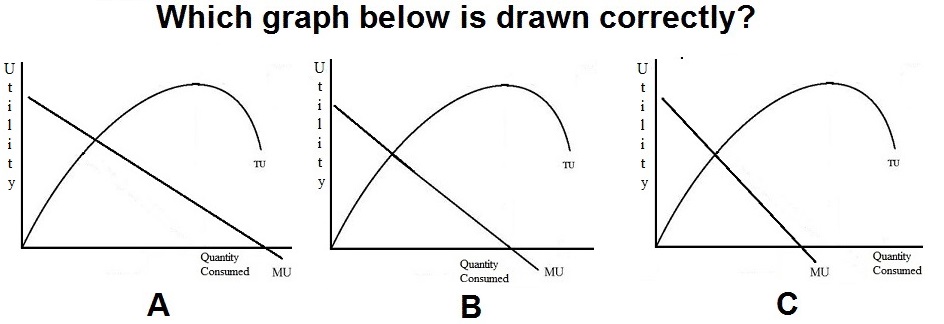
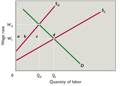
1a Key Graphs |
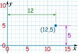
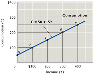
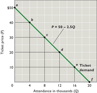
Any Point on a Graph Represents Two Numbers Direct Relationship Inverse Relationship Calculating Slope |
1a Review Videos |
[3:26 YouTube mjmfoodie] Episode
6: Graph Review NOTE: These are REVIEW videos only. In order to learn the material you must read the assigned textbook readings, watch the assigned lecture videos, and do problems. See the LESSONS link on Blackboard for these assignments. |
![]()
|
1b Introduction |
The "5Es of Economics" are not from the textbook. I borrowed the concept (with many modifications) from another textbook many years ago. I believe it concisely explains the purpose of economics. Also, it begins to introduce students to the economic way of thinking. The economic problem that we all face, that all countries face, that the world faces, is SCARCITY. Economics is the study of how we can reduce scarcity. What I like about the 5Es model is that it shows us that there are only five ways to reduce scarcity. Only five. I call them the "5Es" of economics. For each of the 5Es: This is where you learn that it may be good when the price of plywood increases greatly as the result of a hurricane. And why it might be good when Coca-Cola lays of one fifth of its workforce. Or, that the price of gasoline may be too low. Really! |
1b Something Interesting - Why are we studying this? |
When a hurricane hits the coast of Florida, prices of many necessities like food, water, hotel rooms, gasoline, and even plywood, tend to increase. Some governments try to prevent such price increases and call them "price-gouging". See: http://www.csmonitor.com/1992/0910/10083.html But economists think that such price increases are GOOD for the people ravaged by the hurricane. WHY? Why is it GOOD when the prices of products (like plywood) increase during a natural disaster? See: https://www.masterresource.org/price-gouging-law/defense-price-gouging/ ANSWER: Allocative Efficiency |
1b Assignments: Readings |
Syllabus On-Campus / Syllabus Online 5Es online reading (VERY IMPORTANT!) Ch. 3: "Efficient Allocation" pp. 58-59 Ch. 3 and 6: "Diminishing Marginal Utility" pp. 49 and 117 Ch.1, Appendix on Graphing |
1b Assignments: Video Lectures |
REVIEW OF GRAPHING CONCEPTS 1.2.1 Using Graphs to Understand Direct Relationships 9:50 [MyNotes] OPTIONAL: MATH, ALGEBRA, AND GEOMETRY FOR ECONOMICS STUDENTS How to Multiply and Divide Fractions in Algebra for Dummies (YouTube fordummies 1:50) |
Readings:
Topics:
|
Video Lectures: [login] [notes]
|
|
Must Know / Outcomes:
|
Discussion Questions:
|
The 5Es of Economics
1c Scarcity and Budget LinesLesson Introduction: So, do you agree that it is GOOD for the people of Florida if, after a hurricane strikes, the price of plywood (or other products) increases from $10 a sheet to $30 a sheet? Or, that it was GOOD when the Coca-Cola company (or other companies) layed off 6000 workers as they did in the year 2000 assuming that they could still produce the same quantity, but with fewer workers? Even if you do not agree, do you understand that these things will reduce scarcity and increase society's satisfaction? In chapter five we will learn why the prices of gasoline, soda pop, and junk food, may be TOO LOW. (Isn't this fun?) Lesson 1c introduces our first graphic MODEL: the budget line. For many students microeconomics is a difficult course. I think there are two reasons for this. First, we will learn theories or models, rather than facts. Facts are easy to memorize. Theories or models have to be learned and practiced. And second, we will express our theories or models on graphs, and many students do not like graphs. If you want to be successful in this course you must learn to use our graphical models. You must be able to draw the graphs correctly from memory, you must understand what each line on the graph represents, and you must know why each line has the shape that it does. For each graph be able to: DEFINE, DRAW, DESCRIBE its shape. Be sure to study the graphs in the textbook carefully and plot all the graphs in the yellow pages. Finally, an easier way to view graphs is to remember that each point on a graph represents two numbers. Find a point on a graph, then find the two number from the graph's axes. Note: not all models are graphs. For example, the 5Es of Economics is a model of the issues studied by economists.
Key Graphs: Budget Line Budget Line: Income Decreases Budget Line: Price Decreases |
1d Making Choices: Production Possibilities Curve (PPC) and Benefit Cost Analysis (BCA)Lesson introduction: Here we will study our second graphical model: the Production Possibilities Curve (PPC), and we then will learn a tool for making decisions that we will use throughout the course: Benefit-Cost analysis (BCA). Basically what we are doing is setting the stage for making economic decisions. Remember: economics is the social science concerned with how we choose to use our limited resources to maximize society's unlimited wants, or, how we make decisions. The production possibilities curve will show us that we must make choices and all choices have costs. Economists call these "opportunity costs". ALL COSTS IN ECONOMICS ARE OPPORTUNITY COSTS. Whenever we discuss the "costs" of doing something we will mean the complete opportunity cost. Benefit-cost analysis (BCA) is a model that explains how to make the best decision possible. BCA means we should select all options where the marginal benefits (MB) are greater than the marginal costs (MC) -- up to where MB = MC. When the MB = MC then we have made the best decision possible. NOTE: "marginal" means "extra" or "additional". So to make the best decision possible select all options where the extra benefits that you get from the decision are greater than the extra costs of the decision. One more thing: to make the best decisions we look only at MARGINAL costs and benefits and we ignore FIXED, or SUNK, costs (i.e. ignore things that will not change no matter what choice is made). We will use BCA many times throughout this course. In chapter 6 we will use BCA to decide how much to buy to maximize our satistisfaction. In chapters 8-11 we will use it to decide how much to produce to maximize profits. In chapters 12 and 13 we use BCA to decide how many to hire to maximize profits (Ch. 12 and 13). Notice that economists look at EXTRA benefits and EXTRA costs. We call this "thinking on the margin". Students are used to thinking about TOTAL benefits and TOTAL costs. We do not want total benefits to equal total costs, but we do want MB to equal MC. You probably know that it is best if the total benefits are a lot higher than total costs. What you will learn is that when MB = MC, then the difference between total benefits and total costs will be the greatest. Be sure you understand BCA! What is the connection between the PPC and BCA? Well, when studying the PPC you will learn the important concept of "opportunity cost". Learn the definition well. Since all costs in economics are opportunity costs, then when using BCA, "marginal costs" mean the additional opportunity costs.
Reading: Topics: Outcomes / Must Know: PPC Benefit Cost Analysis KEY TERMS: production possibilities, necessity
of choice, law of increasing costs, concave to the
origin, opportunity cost, constant cost,
benefit-cost analysis (marginal analysis), economic
growth, consumer goods, capital goods, shrinking
PPC, nonproportional growth, marginal costs (MC),
marginal benefits (MB), MB=MC Rule, sunk (fixed)
costs Discussion Questions A March 2013 blog post written by Utah
Avalanche Center Director Bruce Tremper . . .
Tremper says airbags are providing a false
sense of security, leading more skiers into
high-consequence terrain, and thus decreasing
the effectiveness of said
airbag. "Don't cry over spilt milk " If you are deciding
whether or not to come to class today, why does it
not matter that you have already paid tuition? Why
is the fact that you have paid tuition irrelevant
when trying to decide whether to attend class today
or skip? Key Graphs: Achieving the Potential: Prod. Efficiency and
Full Employment Increasing the Potential: Economic Growth Benefit-Cost Analysis: Graph: best quantity =
200,000 pizzas |
2a Market Economies and TradeLesson Introduction: One reason why I use our textbook is because they have a chapter on market economies and they used to have a chapter on command economies (now just a small section). In this lesson we find out for the first time that competitive market economies are efficient, both allocatively and productively. This is the result of the "invisible hand" of capitalism. This is a general theme for the whole course that we will discuss again in chapters 3, 5, and 8-13. Many textbooks simply assume that students know what a capitalist economy (market economy) is because we live in one here in the United States. But, I learned long ago that students do not understand the characteristics of captialism nor the benefits of, or the problems with, market economies. All over the world countries are moving away from command economies toward a market economy. Why? We will learn it is because market economies are better at achieving allocative and productive efficiency, and economic growth, but they do seem have a problem with equity and at times full employment. One characteristic of a market economy is a limited role for governement. Periodically we will discuss just WHAT IS the economic role of government? What should the government do, or not do? This is where Republicans and Democrats seem to have a fundamental disagreement, but I think they agree more than they believe. Remember this: the economic goal of society is to maximize its satisfaction (reduce scarcity as much as possible). And they do this by achieving the 5Es. The economic role of government then ALSO should be to achieve the 5Es. We will return to this issue of the economic role of government at different times thoughout the course. Our first discussion of this economic role for government will be FREE TRADE. Should the United States have free trade with other countries like Mexico and China, or should the government impose trade restrictions? We will examine this question by using the production possibilities model that we learned in chapter 1.
|
3a DemandLesson introduction: If the price of pizza goes up, what happens to the demand for pizza? . . . . . . . . . . . . . . . . . . . NOTHING! Nothing happens to the demand for pizza if the price changes! The next three lessons introduce the demand and supply model for explaining how prices arise and change in a market economy. Learn these lessons well. Do the assigned problems. Draw the graphs in the yellow pages and while you are reading and studying. DRAW GRAPHS! Get used to using the graphs to help you answer questions. If you are avoiding drawing the graphs you will do poorly and not get the practice that you need to learn the concept. Be sure to LABEL the axes of every graph that you draw. So why doesn't the demand for pizza change if the price changes? Because economists have a different definition of "demand". Demand is NOT the quantity that we buy. If the price of pizza goes up we will buy less, but that is not what "demand" means in economics. Economists tend to be precise with their definitions and sometimes their definitions are different than the more commonly used definitions. Things like "scarcity", "investment", "cost", "demand", and "supply", have different definitions in economics than what you may already know. Learn our definitions! Demand is not how much we buy. Demand has a different definition in economics. "Demand" means the "demand graph". Remember, that econmists use models (like the supply and demand model) to simplify the real world. They do this by isolating certain variables from all the clutter found in reality. Then by changing one variable at a time economists can see what effect it will have. In this lesson we will learn the economic definition of DEMAND and plot the demand graph. Then, we will look at one variable at a time to see what effect they have on the demand curve. We call these variables the "non-price determinants of demand". They are: Pe, Pog, I, Npot, T (P,P,I,N,T). LEARN THEM! LEARN THEM WELL! Know how each one affects the demand curve. Be sure to do the yellow pages.
Key Graphs:
|
3b SupplyLesson Introduction: If the price of pizza goes up what happens to the SUPPLY of pizza? . . . . . . . . . . NOTHING! A change in the price of a product does not affect its supply, or its demand. When the price goes up the QUANTITY SUPPLIED will increase, but the supply does not change. Learn the difference between "supply" and "quantity supplied". "Supply" does NOT MEAN the quantity available for sale. Supply has a different definition in economics. "Supply" means the "Supply graph". So what would cause the supply graph, or supply itself, to change? Those things that cause supply to change are called the "non-price determinants of supply". They are: Pe, Pog, Pres, Tech, Tax, Nprod (P,P,P,T,T,N). See the Yellow Pages. Remember, the goal of chapter 3 is to learn a model that will help us understand why prices are what they are and why prices change. In the next lesson we will put demand and supply together and use the model (graph) to find the prices of products. Then, and more importantly, we will see what causes prices to change. If you hear on the.news, or read in your news app, that the price of gasoline is going down, we will be able to explain WHY. The causes of changes in prices of products are the five non-price determinants of demand (Pe, Pog, I, Npot, T) and/or the six non-price determinants of supply (Pe, Pog, Pres, Tech, Tax, Nprod.). Whenever you hear that the price of something is changing think of these 11 possible causes.
Key Graphs:
|
3c Market Equilibrium and EfficiencyLesson introduction: We are going to learn two very important things in this lesson. First, we will put demand and supply together and learn how to use the model to to see why products have the prices that they do. Then, and more importantly, we will see what causes prices to change. If you hear on the news or read in your news app ,that the price of gasoline is going down, we will be able to explain WHY. The causes of changes in prices of products are the five non-price determinants of demand (Pe, Pog, I, Npot, T) and/or the six non-price determinants of supply (Pe, Pog, Pres, Tech, Tax, Nprod.). Whenever you hear that the price of something is changing think of which of these 11 possible causes have changed, draw the graph and shift the appropriate demand and/or supply graph, and the graph will show the price changing. Second, after we learn that in a competitive market economy the interaction of demand and supply will determine what the prices of products will be and how much people will buy at that price, we will ask: Is this the allocatively efficient quantity and price? Our goal is to show that in a competitive market the price will change until allocative efficiency is achieved. In chapter 2 we learned that markets are allocatively efficient. This means they will produce the quantity of goods that maximizes the society's satisfaction. After studying chapter 3 we will bew able to show the allocatively efficient price and quantity on a graph. Competitive markets are efficient.
Key Graphs:
|
5a Government Interference in Markets and Market Failures (Negative Externalities)Lesson introduction: In lesson 3c we learned that competitive markets are efficient and we learned two models to show that markets are efficient: (1) MSB = MSC, and (2) maximum consumer plus producer surplus. You must understand these models to understand chapter 5. In chapter 5 we learn that SOMETIMES markets are NOT efficient. When are product markets not efficient?
In this lesson we also will begin our look at the role of the government in a market economy. This would be a good time to review chapter 2. In chapter 2 we learned that there is a limited role for government in market economies. We learned in lesson 3c that markets are efficient, so there is little need for the government. In this lesson we will see what happens if the government interferes in markets. We will learn that sometimes governments will set prices (price ceilings and price floors), rather than letting the market set the price. In other words: SOMETIMES GOVERNMENTS CAUSE ALLOCATIVE INEFFICIENCY. (This is the plywood after a hurricane example discussed in the 5Es reading in lesson 1b.) Then we will begin to look at examples of when the markets on their own fail to achieve allocative efficiency and examine what the government can do to correct these market failures. SOMETIMES MARKETS BY THEMSELVES ARE INEFFICIENT and the government may try to modify the market to help it achieve allocative efficiency. There are three MARKET FAILURES that we will look at in chapter 5. A "market failure" occurs when the market fails to achieve allocative efficiency. In lesson 5a we look at the market failure caused by negative externalities - when the supply curve does not include all of the costs to society of producing and consuming the product. Then in lesson 5b we look at the market failures caused by positive externalities and public goods. We will assume that businesses will always produce the profit maximizing quanitity since their goal is to maximize profits. The profit maximizing quantity is also the equilibrium quantity that we studied in chapter 3, when the Qs = Qd. This is WHAT WE GET. We get whatever they produce and they will produce the quantity that gives them the biggest profits. The goal of business is not to be efficient. Their goal is to maximize their profits. If a business can make larger profits by being inefficient then they will be inefficient. Or if they can make larger profits by being efficient they they will be efficient. The main point is that efficiency is not their goal, rather, maximizing profits is their goal. The allocatively efficient quantity is what society wants. We learned at the end of chapter 3 that allocative efficiency occurs at the quantity where MSB = MSC. This is WHAT WE WANT. We want to maximize our satisfaction and we learned in chapter 1 that this occurs when we achieve the 5 Es. Allocative efficiency is one of the 5 Es. When the profit maximizing quantity equals the allocatively efficient quantity then markets are efficient . This means that profit maximizing businesses are producing the quantity that maximizes society's satisfaction. WHAT WE GET = WHAT WE WANT. This is the INVISIBLE HAND of capitalism that was discussed in chapter 2. It's as if there is an invisible hand guiding businesses to not only make decisions that maximize their profits, but also to maximize society's satisfaction. As if they don't even know it is happening. When markets fail to achieve allocative efficiency, the profit maximizing quantity (WHAT WE GET or the equilibrium quantity from chapter 3) is not the same as the allocatively efficient quantity (WHAT WE WANT or the quantity where MSB=MSC). Since one of the economic goals of government is to help the economy achieve efficiency, governments often get involved to correct for market failures. If the market produces too much (negative externalities cause allocative inefficiency because of an overallocation of resources) the government tries to get it to produce less. If the market produces too little (positive externalities and public goods causing allocative inefficiency resulting in an underallocation of resources) the government tries to get it to produce more.
Key Graphs: Price Ceiling (causes a shortage) Price Floor (causes a surplus) Negative Externality Negative Externality and Taxes |
5b Market Failures Continued (Positive Externalities and Public Goods)Lesson introduction: We have learned that competitive markets are usually efficient. This is one of the benefits of a market economy or capitalism (chapter 2) . But sometimes even markets can be allocatively inefficient. In lesson 5a we learned that when negative externalities exist, a market will produce too much of a good or service (an overallocation of resources) and therefore the government should tax the product (like gasoline taxes) to get consumers to buy less, i.e. without the tax the price of gasoline is too low. In this lesson we will look at two other market failures, but this time the market produces too little (an underallocation of resources) because the demand curve for the product does not include all of the benefits. This occurs when there are positive externalities and when there are "public goods". Be careful - remember - economists often change the definitions of words. Public schools and public parks are not public goods according to our definition. Since markets produce too little when there are negative externalities or public goods, the goal of government is to increase production. In later chapters (10 and 11) we will discuss another market failure: the lack of competition. If a market is not competitive, like when it is a monopoly or an oligopoly, then profit maximizing businesses will produce less than the allocatively efficient amount. The invisible hand of capitalism does not work well if the market is not competitive.
|
Positive Externalities
Positive Externalities and the Role of Government: Increase Demand
Positive Externalities and the Role of Government: Increase Supply
|
4a Something Interesting (Why are we studying this?) In 2012 there was a severe drought in the US corn growing region. In 2014 the weather was great and the corn crop was at a record high. In which year did farmers make the most money? They made more in 2012 when the weather was bad !!! After studying this lesson you should understand why good farming weather results in low farm incomes and bad farming weather results in high farm incomes. Really! See:
ANSWER: The answer to this paradox is that the demand for corn and soybeans is price INELASTIC. You will learn that bad weather causes the price of crops to increase whch causes farm incomes to increase and good weather causes the price of farm corps to decrease causing incomes to decrease BECAUSE THE DEMAND FOR CORN AND SOYBEANS IS PRICE INELASTIC. |
Readings:
Topics:
|
Video Lectures: [login] [notes]
|
Must Know / Outcomes:
|
Discussion Questions:
|
Key Graphs
4b Other Types of ElasticityLesson Introduction: Elasticity tells us HOW MUCH one variable changes in response to a change in another variable. Chapter 3: If price increases what happens to the
quantity demanded? We will study four different types of elasticity: 1. price elasticity of demand (lesson 4a)
Key Graphs: |
6a Consumer Decisions: Utility MaximizationLesson Introduction: When I go into the grocery store why do I buy 12 cans of pop, 3 frozen pizzas, and 1 pound of hamburger? Why don't I buy 12 pounds of hamburger and 1 can of pop? In this lesson we will use benefit-cost analysis to understand why we buy what we do. We will calculate the marginal benefits (MB) of consuming something and the marginal costs (MC) of consuming something. Remember: all costs in economics are opportunity costs. If our goal is to maximize our satisfaction we will consume the quantity of goods and services where MB = MC. First, we will examine the benefits we get from consumption. Economists call these benefits "utility". We will calculate and graph total utility (TU) and marginal utility (MU). As always, be sure you understand the SHAPES of these graphs. Remember: Define, Draw, Describe. Then, we will use the utility maximizing rule, to calculate how much we should buy in order to maximize our satisfaction (utility). Be sure that you can see that the utility maximizing rule is really just a version of benefit cost analysis, MB=MC. If I am thinking about going skiing today, the MB would be the extra utility that I get from a day of skiing: MBskiing = MUskiing. Since all costs are opportunity costs, the marginal cost of skiing would be the utility that I would lose because I am not doing something else like going to a movie with my wife: MCskiing = MUmovie Finally, why do we divide the MU by the price? It doesn't make sense to compare a $45 ski ticket with a $12 movie ticket. By dividing by price we end up comparing $1 worth of skiing with $1 worth of a movie. So, to maximize my utility I should go skiing and go to movies with my wife so the: MUskiing/Pskiing= MUmovie/Pmovie. So even though MUx/Px = MUy/Py looks different than MBx=MCx, it is really the same thing. Be sure you do the exercises in the yellow pages.
Key Graphs: Total Utility (TU) and Marginal Utility (MU)
WHY? |
7a Economic Profit and the Production FunctionLesson Introduction: In chapters 7, 8, 9, 10, and 11 we will be at looking the producer decision of HOW MUCH TO PRODUCE. We will use benefit cost analysis (MB=MC) to find the profit maximizing quantity or WHAT WE GET. Once we know how much businesses will produce, we will ask: Is this quantity efficient (both allocatively and productively)? To find the profit maximizing quantity we will use benefit-cost analysis: MB=MC. So, what are the extra benefits of producing one more unit of output? How do businesses benefit when they produce one more? Well, they get more money, called revenue. Even if they are earning losses, they receive more revenue when they sell more. The extra revenue that businesses get when they produce and sell one more unit is their marginal revenue (MR). This is the MB of producing one more. But there are also extra costs of producing one more unit of output. We call these the marginal costs (MC). When MR=MC (MB=MC) their profits will be maximized. NOTE: when MR=MC profits are not necessarily zero, but they are as large as possible. We will calculate these profits in chapters 8, 9, 10, and 11. In this chapter, chapter 7 we begin by looking at the MC. Then in chapters 8, 9, 10, and 11 we add the MR. In chapter 7 we will introduce three new sets of graphs. First (lesson 7a) we will look at the production function thast shows how output changes when we add more resources. We will then (lesson 7b) use the production function graph to understand the SHAPES of the other two sets ofgraphs. The two sets of cost graphs show us what happens to costs when we produce more. These two sets of cost graphs are the total cost graphs (TC, TVC, and TFC) and the average cost graphs (ATC, AVC, AFC, and MC).
KEY GRAPHS: The Production Function: Total Product (TP), Average Product (AP), and Marginal Product (MP)
WHY? |
7b Production Costs in the Short RunLesson Introduction: OK. Now that we know about (1) specialization and teamwork, (2) getting crowded, and (3) overcrowded, from lesson 7a, that is, we know why the TP curve has the shape that it does, we are ready to look at the graphs that we will be using most in this class: the cost curves (both total and average). Remember, we are studying economic costs so that we can calculate the MC - the extra costs of producing one more unit of output. In chapters 8, 9, 10, 1nd 11 we will combine MC with MR (the extra benefits of producing and selling one more unit of output ) so that we can find the profit maximizing quantity of output, or the quantity where MR=MC. This is WHAT WE GET. The costs curves show us how costs change with output. The production function in lesson 7a showed us how output changes when we add more resources. They are related. We studied the production function so that we could learn about (1) specialization and teamwork, (2) getting crowded, and (3) overcrowded, because these concepts will help us understand the shapes of the cost curves. Remember: whenever we learn a new graph we must understand it shape (For all graphs: DEFINE, DRAW, DESCRIBE its shape).
Key Graphs:
WHY? |
7c Production Costs in the Long RunLesson Introduction: In lesson 7c we claculated and graphed SHORT RUN costs when the size of the factory was fixed (did not change). chapter 4). Here we will learn how costs change in the LONG RUN. In the long run we can change the size of the factory. Be sure that you can define "short run" and "long run". As always, be sure you know why the long run ATC curve has the shape it does; For all graphs: DEFINE, DRAW, DESCRIBE the SHAPE. Note that in the next unit (unit 3) we will use long run graphs to find the allocatively efficient quantity and the productively efficient quantity.
Key Graphs: Economies of Scale over a wide range of output
|
|
8/9a Something Interesting (Why are we studying this?) -- Are businesses efficient?
ANSWER: Whenever you are asked questions like:
the first thing you do is calculate MR and MC. Then, as long as the firm earns more (MR) than it costs (MC) they will produce. They will produce ALL where MR>MC, up to where MR=MC, but never where MR<MC. |
Readings:
Topics:
|
Video Lectures: [login] [notes]
|
Must Know / Outcomes:
|
Discussion Questions:
|
Key Graphs:
Pure Competition: Short Run Earning
Losses Pure Competition: Short Run Shut Down
Pure Competition: Short Run Earning
Profits
8/9b Pure Competition - Long Run Equilibrium and Efficiency - Are Businesses Efficient?Lesson Introduction: Again, we return to the central issue of economics: reducing scarcity (the 5Es). In chapters 9, 10, and 11 we will see if industries are (1) allocatively efficient, and (2) productively efficient, in the long run. This would be a good time to review the 5Es online reading from lesson 1b and reacquaint yourself with the definitions and examples of allocative and productive efficiency. Allocative efficiency means producing the mix of goods and services that maximize society's satisfaction and productive efficiency means producing at a minimum cost. What else do we know? In chapter 1 we learned about benefit-cost analysis (marginal analysis). From chapters 3 and 5 we know that we find the allocatively efficient quantity where MSB = MSC and where consumer plus producer surplus are maximized. In chapter 4 we learned the definitions of short run and long run. In chapters 9, 10, and 11 we will put all of this together to see if businesses are efficient. Of course we do not have time to study every individual business or industry, so we will examine the efficiency of four groups of industries or the four product market models. In chapter 2 we learned that competitive markets are efficient. In chapter 8 we learned the characteristics of competitive markets and how competitive businesses find the profit maximizing quantity to produce (where MR=MC or WHAT WE GET). Here, we will learn that since there are no barriers to entry in the long run the competitive markets will produce the allocatively efficient quantity that people want at the lowest possible cost (productive efficiency). Be sure to see the "Three Rules and Four Models" Yellow (Blue) Page. Finally, once we learn that the allocatively efficient quantity occurs where P = MC, we will look at ways this might be used to improve the allocation of resources and reduce scarcity. (MC Pricing). Never forget this: To maximize profits business will produce the quantity where MR=MC.
Key Graph Pure Competition: Long Run Equilibrium |
10a Monopoly: Characteristics and Short-Run Equilibrium - Are Businesses Efficient?Lesson Introduction: We learned in lesson 2a that competitive markets are efficient (except when there are externalities or public goods - ch.5). But what happens if markets are NOT competitive? We said that competition is the "invisible hand" that forces businesses to be efficiency. If the market is not competitive we will not get the efficient quantity. This means that the profit maximizing quantity that businesses will produce (WHAT WE GET) will not be the same as the allocatively efficient quantity that society wants (WHAT WE WANT). Remember the word "competition" has a different meaning in economics. This is NOT the competition that occurs between Ford and Chevrolet. "Competition" in economics means there are many buyers and sellers in the market so that firms have no influence over the price; i.e. they are price takers. Much of the business world is not competitive, and therefore, not efficient. In this lesson we will look at monopolistic industries - industries with only one firm. There are few pure monopolies. Even though there are few true monopolies they do exist, but we will also study monopolies because most firms are a combination of competition and monopoly. For each of the four product market models (chapters 8-11), including monopolies, you should use the following general outline to guide your studying: General Outline for Each Product Market Model: 1. Know the model's characteristics and examples (See the "Ch. 8 - 4 PRODUCT MARKET MODEL" quiz on our Blackboard site.) Never forget this: To maximize profits business will produce the quantity where MR=MC.
Key Graphs: Monopoly: Short Run Earning Losses Monopoly: Short Run Shut Down |
10b Monopoly: Long-Run, Efficiency, Price Discrimination, and Regulation - Are Businesses Efficient?Lesson Introduction: In chapter 9 we learned that in the long run purely competitive firms are both allocatively and productively efficient. They maximize society's satisfacton. In lesson 10a we learned how find the quantity produced by monopolies. Here in lesson 10b we will learn if that quantity that we get, the profit maximiing quantity is the efficient quantity. Are monopolies efficient? Are businesses efficient? In chapter 9 we also learned that if purely competitive firms have short run profits, then in the long run new firms will enter. This will increase the supply of the product because if the number of producers increases then supply increases (chapter 3). When supply increases it causes the price to drop and this will reduce the profits of the firms. This will continue to happen until there are just normal profits. In the long run, purely competitive firms earn only normal (zero) profits BECAUSE THERE ARE NO BARRIERS TO ENTRY. So, what about monopolies? In this lesson we will learn that SINCE MONOPOLIES DO HAVE BARRIERS TO ENRTY (entry is blocked) they will earn economic profits in the long run, Also, at the profit maximizing quantity (what we get) monopolies will be both allocatively and productively INEFFICIENT. When monopolies produce the quantity that maximizes their profits they will be producing less than the allocatively efficient quantity (underallocation of resources) AND they will not be producing at the lowest possible cost per unit (productive inefficiency). Next, we will look at PRCE DISCRIMINATION. What if instead of charging the same price to all customers, a monopoly charged different prices to different customers for the same product? We will learn that if monopolies price discriminate then they will produce more and the market will be MORE allocatively efficient. Finally, since momopolies are inefficient the government usually prevents them from forming (anti-trust laws), but sometimes the government will allow a monopoly to exist if it is in the public interest, like when it is a natural monopoly, but they will then regulate it, i.e. set its price. So in this lesson we will study three things: 1. monopolies are allocatively and productively inefficient
Key Graphs: Monopoly: Long Run Equilibrium Regulated Natural Monopoly Monopoly with Perfiet Price
Discrimination |
11a Monopolistic Competition - Are Businesses Efficient?Lesson Introduction: Competitive firms are efficient and monopolies are inefficient, but there are few if any cpurely ompetitive markets or purely monopolistic markets (monopolies). So what happens in the real world? Are businesses efficient? We learned that competitive firms earn zero long run profits because there are no barriers to entry and monopolies do earn long run profits because entry is blocked. What about monopolistically competitive markets where there are LOW BARRIERS? What about oligopolistic markets where there are HIGH BARRIERS? Guess what? If there are low barriers firms will earn zero long run profits (monopolistic competition) and if there are high barriers firms will earn long run economic profits (oligopolies). What about efficiency? We will learn that both monopolistically competitive firms and oligopolies are inefficient but not to the same degree. Monopolistically competitive frms are only slightly inefficient and they do provide society some additional benefits, but oligopolies are very inefficient and are closely watched by the government. General Outline for Each Product Market Model: 1. Know the model's characteristics and examples (See the "Ch. 8 - 4 PRODUCT MARKET MODEL" quiz on our Blackboard site.) Never forget this: To maximize profits business will produce the quantity where MR=MC.
Key Graph Monopolistic Competition in Long Run Equilibrium |
11b Oligopoly - Are Businesses Efficient?Lesson Introduction: Oligopolies are industries with just a few firms because there are high barriers to entry. So do they earn long-run profits (YES) and are they efficient (NO)? Oligopolies are more complex than the other three models. Instead of one model to explain how oligopolies determine price and quantity we will have four: 1. kinked demand model General Outline for Each Product Market Model: 1. Know the model's characteristics and examples (See the "Ch. 8 - 4 PRODUCT MARKET MODEL" quiz on our Blackboard site.) Never forget this: To maximize profits business will produce the quantity where MR=MC.
Oligopoly Kinked Demand Long Run
Equilibrium Oligopoly Game Theory |
|
12a Something Interesting (Why are we studying this?) Why are people paid differently? (Look at the websites below.)
ANSWER: The supply and demand for labor helps explain why different people and different jobs receive different wages. But there are also other factors that we will need to explore. We will end up with 8 to 10 different labor market models that will help us answer this question. |
Readings:
Topics:
|
Video Lectures: [login] [notes]
|
Must Know / Outcomes:
|
Discussion Questions:
|
Key Graphs
Competitive Labor Market in a Imperfectly
Competitive Product Market
Competitive Labor Market in a
Competitive Product Market
13a Wage Determination (Labor Markets)Lesson Introduction: Eight Labor Market Models 1. Competitive labor market in a competitive product market For EACH model know the following: 1. assumptions, characteristics, and examples You will find a summary of each of these eight (actually ten) models in our Yellow Pages. It is strongly recommended that you study these summaries. REMEMBER: to find the profit maximizing quantity of workers to hire firms will continue to hire up to the point where MRP = MRC. So for any questions that ask "how many will be hired?" or "what will the wage be?" the first thing you do is calculate MRP and MRC and then hire all where the MRP is greater than MRC (MRP > MRC) up to where MRP = MRC.
Key Graphs: Comp. Labor Market and Comp. Labor Market and Monopsony Union: Increase Demand Union: Craft (Exclusive) Union: Inclusive (Industrial) Union: Bilateral Monopoly Minimum Wage Models: | | | Min. Wage Traditional Model: Min. Wage in a Monopsony: Does the Minimum wage help the poor? YES if the demand for labor is inelastic because
total income increases from 0ADF to 0BCE Does the Minimum wage help the poor? NO if demand for labor is elastic because total
income decreases from 0adf to 0bce |
20a Income Inequality and DiscriminationLesson Introduction: The gap between the rich and the poor is getting wider and income inequality has become an important political issue. We will learn that the 85 richest people on Earth now have the same amount of wealth as the bottom half of the global population. 85 people have the same amount of wealth as the poorest 3.5 billion (3,500,000,000) ! We will first look at some data on the distribution of income and learn how to measure it. Then we will learn two models concerning income distribution: 1. The Case for Equality Model: Maximizing Total Utility This is the President Obama Example of lesson 1b (fig. 20.3) and The Yellow Pages have one page summaries of each of these models. You should find them and study them.
Key Graphs: Lorenz Curve |
22a ImmigrationLesson Introduction: Immigration is another labor issue that has become an important political topic. We will first study some historical data on U.S. immigration then we will look at two immigration models: 1. a simple immigration model showing the "Impact on Wage Rates, Efficiency, and Output", and The Yellow Pages have one page summaries of each of these models. You should find them and study them.
Key Graphs: Simple Immigration Model |
[MyNotes]